Sensitivity, stability, and residuals

A discrepancy can originate in the mathematical problem, the selected algorithm, or its implementation. This tutorial uses controlled examples to separate problem sensitivity from algorithmic error and to show why residual and forward error answer different questions.

This activity accompanies Module 4: Conditioning And Numerical Stability.

Download the executable Jupyter notebook Open in Google Colab

Learning goals

After this experiment, you should be able to:

• estimate directional input-to-output amplification;
• distinguish sensitivity that persists in high precision from algorithmic finite-precision error;
• compare algebraically equivalent algorithms using forward and backward error;
• compute a scaled residual for a linear system;
• explain how small backward error can coexist with large forward error;
• record which evidence supports each diagnosis and which limitations remain.

Prerequisites

Read Module 3: Measuring And Comparing Numerical Error or complete the comparison criteria across scales activity first. This tutorial assumes that you can interpret relative error and a stated norm. It introduces conditioning and stability rather than assuming them.

Outline

1. Perturb two related linear systems in high precision.
2. Estimate observed amplification as the systems become nearly dependent.
3. Compare two algorithms for the same quadratic root.
4. Measure forward and coefficient backward error.
5. Construct a small-residual, large-forward-error candidate.
6. Record the diagnosis and limitations.

Set up the sensitivity problem

For nonzero \(\delta\), consider the dimensionless system

\[ x_1+x_2=2, \qquad x_1+(1+\delta)x_2=2+\delta. \]

Its exact solution is \((1,1)\). The code uses 80-digit decimal arithmetic so that the observed amplification is not an accidental binary64 effect. The maximum norm is used for both input and output changes.

from decimal import Decimal, getcontext, localcontext
import math


getcontext().prec = 80
D = Decimal


def max_norm(values):
    """Return the maximum absolute component."""
    return max(abs(value) for value in values)


def solve_two_equation_system(delta, second_rhs_perturbation=D(0)):
    """Solve the constructed system analytically in Decimal arithmetic."""
    first_rhs = D(2)
    second_rhs = D(2) + delta + second_rhs_perturbation
    x2 = (second_rhs - first_rhs) / delta
    x1 = first_rhs - x2
    return [x1, x2]


def sensitivity_diagnostics(delta, perturbation):
    """Return relative changes and observed directional amplification."""
    base_rhs = [D(2), D(2) + delta]
    input_change = [D(0), perturbation]
    base_solution = solve_two_equation_system(delta)
    perturbed_solution = solve_two_equation_system(delta, perturbation)
    output_change = [
        perturbed - base
        for perturbed, base in zip(perturbed_solution, base_solution)
    ]

    relative_input_change = max_norm(input_change) / max_norm(base_rhs)
    relative_output_change = max_norm(output_change) / max_norm(base_solution)
    observed_amplification = relative_output_change / relative_input_change
    return {
        "base_solution": base_solution,
        "perturbed_solution": perturbed_solution,
        "relative_input_change": relative_input_change,
        "relative_output_change": relative_output_change,
        "observed_amplification": observed_amplification,
    }


input_perturbation = D("1e-16")
print(f"decimal precision: {getcontext().prec} digits")
print(f"second right-hand-side perturbation: {input_perturbation:.1E}")

decimal precision: 80 digits
second right-hand-side perturbation: 1.0E-16

Compare separated and nearly dependent systems

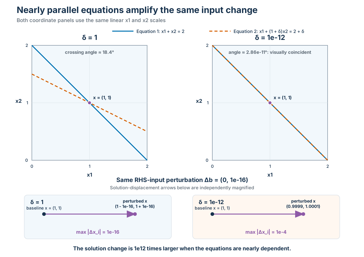
Predict how the same right-hand-side perturbation affects the solution when \(\delta=1\) and when \(\delta=10^{-12}\).

conditioning_results = {}

print(
    f"{'delta':>12s}  {'relative input':>16s}  "
    f"{'relative output':>16s}  {'amplification':>16s}"
)
for delta_text in ["1", "1e-12"]:
    delta = D(delta_text)
    diagnostics = sensitivity_diagnostics(delta, input_perturbation)
    conditioning_results[delta_text] = diagnostics
    print(
        f"{delta:.1E}  "
        f"{diagnostics['relative_input_change']:16.3E}  "
        f"{diagnostics['relative_output_change']:16.3E}  "
        f"{diagnostics['observed_amplification']:16.3E}"
    )
    print(f"  perturbed solution: {diagnostics['perturbed_solution']}")

       delta    relative input   relative output     amplification
1.0E+0         3.333E-17         1.000E-16          3.000E+0
  perturbed solution: [Decimal('0.9999999999999999'), Decimal('1.0000000000000001')]
1.0E-12         5.000E-17          1.000E-4         2.000E+12
  perturbed solution: [Decimal('0.9999'), Decimal('1.0001')]

The separated system amplifies this direction by about 3. The nearly dependent system amplifies it by about \(2\times10^{12}\): a relative input change near \(5\times10^{-17}\) produces a relative output change of \(10^{-4}\). This is problem sensitivity observed in high precision.

Exercise: vary the separation

Change exercise_delta and predict the amplification before running the cell. Try powers of ten between 1 and \(10^{-12}\). Which quantity in the equations suggests the trend?

exercise_delta = D("1e-6")  # Try 1, 1e-4, 1e-8, or 1e-12.
exercise_diagnostics = sensitivity_diagnostics(
    exercise_delta,
    input_perturbation,
)

print(f"delta:                  {exercise_delta:.1E}")
print(
    "relative input change:  "
    f"{exercise_diagnostics['relative_input_change']:.3E}"
)
print(
    "relative output change: "
    f"{exercise_diagnostics['relative_output_change']:.3E}"
)
print(
    "observed amplification: "
    f"{exercise_diagnostics['observed_amplification']:.3E}"
)

delta:                  1.0E-6
relative input change:  5.000E-17
relative output change: 1.000E-10
observed amplification: 2.000E+6

Check the sensitivity trend

The exact solution change contains the ratio \(\eta/\delta\). The sweep below checks how that factor appears in the relative amplification. One direction is being sampled; this is not a complete worst-case condition-number calculation.

for delta_text in ["1", "1e-4", "1e-8", "1e-12"]:
    delta = D(delta_text)
    amplification = sensitivity_diagnostics(
        delta,
        input_perturbation,
    )["observed_amplification"]
    print(f"delta = {delta:.1E}: amplification = {amplification:.3E}")

delta = 1.0E+0: amplification = 3.000E+0
delta = 1.0E-4: amplification = 2.000E+4
delta = 1.0E-8: amplification = 2.000E+8
delta = 1.0E-12: amplification = 2.000E+12

Define forward and backward error formally

Let \(d\) denote the supplied problem data and let \(S(d)\) be the set of exact solutions. The forward error of a computed result \(\hat{x}\) is

\[ e_{\mathrm{fwd}}(\hat{x};d) = \inf_{x\in S(d)} \rho_X(\hat{x},x). \]

For a unique nonzero exact solution \(x\), a common relative normwise choice is \(\rho_X=\|\hat{x}-x\|_X/\|x\|_X\). With multiple solutions, \(S(d)\) must represent the acceptable solutions or the intended branch. If \(x\) is replaced by a justified numerical reference, the measured value is an estimate of the unknown exact forward error.

The backward error instead measures distance in the data space:

\[ \eta(\hat{x};d) = \inf_{\Delta d\ \text{admissible}} \left\{ \rho_D(d,d+\Delta d) \;:\; \hat{x}\in S(d+\Delta d) \right\}. \]

This definition asks for the infimum of the sizes of admissible input changes that make the computed result exact. It is incomplete unless the allowed changes, preserved structure, norm, and scaling in \(\rho_D\) are stated. For \(Ax=b\) with \(A\) fixed and \(r=b-A\hat{x}\), choosing \(\rho_D=\|\Delta b\|/\|b\|\) gives \(\eta_b=\|r\|/\|b\|\), because \(\hat{x}\) exactly solves \(A\hat{x}=b-r\).

Hold the problem fixed and change the algorithm

Now consider the dimensionless polynomial

\[ p(x)=x^2-10^8x+1. \]

The direct formula subtracts the square root from \(10^8\) to obtain the small root. The reformulation computes the large root using addition, then uses the fact that the product of the roots is one. Both solve the same mathematical problem in the same binary64 format.

The high-precision reference is recomputed with 80 and 100 decimal digits. Their relative difference checks that reference precision is far beyond what this comparison needs.

def decimal_small_root(precision):
    """Compute the small quadratic root at a requested Decimal precision."""
    with localcontext() as context:
        context.prec = precision
        coefficient = D("1e8")
        discriminant_root = (coefficient**2 - D(4)).sqrt()
        return +(coefficient - discriminant_root) / D(2)


reference_80 = decimal_small_root(80)
reference_100 = decimal_small_root(100)
reference_difference = abs(reference_80 - reference_100) / abs(reference_100)

coefficient_float = 1.0e8
discriminant_root_float = math.sqrt(coefficient_float**2 - 4.0)
large_root_float = (
    coefficient_float + discriminant_root_float
) / 2.0
direct_small_root_float = (
    coefficient_float - discriminant_root_float
) / 2.0
reformulated_small_root_float = 1.0 / large_root_float

print(f"80-digit reference:  {reference_80:.18E}")
print(f"100-digit reference: {reference_100:.18E}")
print(f"relative reference difference: {reference_difference:.3E}")
print(f"direct binary64 root:       {direct_small_root_float:.17g}")
print(f"reformulated binary64 root: {reformulated_small_root_float:.17g}")

80-digit reference:  1.000000000000000100E-8
100-digit reference: 1.000000000000000100E-8
relative reference difference: 4.200E-79
direct binary64 root:       7.4505805969238281e-09
reformulated binary64 root: 1e-08

Measure forward and backward error

Forward error compares a candidate with the high-precision root. For the polynomial, use the scaled coefficient backward error

\[ \eta_p= \frac{|p(\hat{x})|} {|\hat{x}|^2+10^8|\hat{x}|+1}. \]

It measures the relative coefficient perturbation needed to make the candidate an exact root under this component-scaled model.

def quadratic_diagnostics(candidate_float, reference):
    """Return Decimal forward, residual, and coefficient backward errors."""
    with localcontext() as context:
        context.prec = 100
        candidate = D.from_float(candidate_float)
        coefficient = D("1e8")
        residual = candidate**2 - coefficient * candidate + D(1)
        forward_error = abs(candidate - reference) / abs(reference)
        backward_scale = (
            abs(candidate**2) + abs(coefficient * candidate) + D(1)
        )
        backward_error = abs(residual) / backward_scale
        return {
            "forward_error": +forward_error,
            "residual": +residual,
            "backward_error": +backward_error,
        }


quadratic_results = {
    "direct": quadratic_diagnostics(
        direct_small_root_float,
        reference_100,
    ),
    "reformulated": quadratic_diagnostics(
        reformulated_small_root_float,
        reference_100,
    ),
}

print(
    f"{'method':>12s}  {'forward error':>16s}  "
    f"{'polynomial residual':>20s}  {'backward error':>16s}"
)
for method, diagnostics in quadratic_results.items():
    print(
        f"{method:>12s}  {diagnostics['forward_error']:16.3E}  "
        f"{diagnostics['residual']:20.3E}  "
        f"{diagnostics['backward_error']:16.3E}"
    )

      method     forward error   polynomial residual    backward error
      direct          2.549E-1              2.549E-1          1.461E-1
reformulated         7.908E-17             7.908E-17         3.954E-17

The direct calculation has roughly 25% forward error and requires a large coefficient perturbation under the stated backward measure. The reformulated calculation has forward and backward errors near binary64 rounding scale. This is evidence about the algorithms because the polynomial, input coefficients, arithmetic format, reference, and metrics are held fixed.

Compare residual with forward error

Return to the nearly dependent system with \(\delta=10^{-12}\). Its exact solution is \((1,1)\). The candidate \((0,2)\) is visibly far away, but calculate its residual and the right-hand-side perturbation that would make it exact.

small_delta = D("1e-12")
exact_solution = [D(1), D(1)]
candidate_solution = [D(0), D(2)]
right_hand_side = [D(2), D(2) + small_delta]

matrix_times_candidate = [
    candidate_solution[0] + candidate_solution[1],
    candidate_solution[0]
    + (D(1) + small_delta) * candidate_solution[1],
]
residual = [
    rhs - product
    for rhs, product in zip(right_hand_side, matrix_times_candidate)
]

relative_forward_error = max_norm(
    [
        candidate - exact
        for candidate, exact in zip(candidate_solution, exact_solution)
    ]
) / max_norm(exact_solution)
relative_rhs_backward_error = max_norm(residual) / max_norm(right_hand_side)
nearby_right_hand_side = matrix_times_candidate

observed_conditioning = conditioning_results["1e-12"][
    "observed_amplification"
]

print(f"exact solution:                  {exact_solution}")
print(f"candidate solution:              {candidate_solution}")
print(f"residual b - A*x_candidate:      {residual}")
print(f"relative forward error:          {relative_forward_error:.3E}")
print(f"relative RHS backward error:     {relative_rhs_backward_error:.3E}")
print(f"nearby right-hand side:          {nearby_right_hand_side}")
print(
    "conditioning estimate * backward error: "
    f"{observed_conditioning * relative_rhs_backward_error:.3E}"
)

exact solution:                  [Decimal('1'), Decimal('1')]
candidate solution:              [Decimal('0'), Decimal('2')]
residual b - A*x_candidate:      [Decimal('0'), Decimal('-1E-12')]
relative forward error:          1.000E+0
relative RHS backward error:     5.000E-13
nearby right-hand side:          [Decimal('2'), Decimal('2.000000000002')]
conditioning estimate * backward error: 1.000E+0

The relative backward error is about \(5\times10^{-13}\), but the relative forward error is one. The candidate exactly solves a nearby system, and this ill-conditioned problem amplifies that small input change. A small residual is therefore evidence of a nearby solved problem, not necessarily of proximity to the desired solution.

Evidence record

A diagnosis should record which object was tested, which metric was used, and what remains unproven. This prevents “ill-conditioned” or “unstable” from becoming an unsupported label.

evidence = {
    "conditioning_experiment": {
        "arithmetic": "Decimal with 80 digits of precision",
        "norm": "maximum norm on dimensionless quantities",
        "input_perturbation": input_perturbation,
        "observed_amplification_delta_1": (
            conditioning_results["1"]["observed_amplification"]
        ),
        "observed_amplification_delta_1e_12": observed_conditioning,
        "limitation": "One perturbation direction, not a full condition number.",
    },
    "algorithm_experiment": {
        "problem": "Small root of x**2 - 1e8*x + 1",
        "reference_check_relative_difference": reference_difference,
        "direct_forward_error": quadratic_results["direct"]["forward_error"],
        "direct_backward_error": quadratic_results["direct"]["backward_error"],
        "reformulated_forward_error": (
            quadratic_results["reformulated"]["forward_error"]
        ),
        "reformulated_backward_error": (
            quadratic_results["reformulated"]["backward_error"]
        ),
        "limitation": "One coefficient set, not a general stability proof.",
    },
    "residual_experiment": {
        "relative_forward_error": relative_forward_error,
        "relative_rhs_backward_error": relative_rhs_backward_error,
        "conclusion": (
            "A small scaled residual does not imply small forward error "
            "for this ill-conditioned system."
        ),
    },
}
evidence

{'conditioning_experiment': {'arithmetic': 'Decimal with 80 digits of precision',
  'norm': 'maximum norm on dimensionless quantities',
  'input_perturbation': Decimal('1E-16'),
  'observed_amplification_delta_1': Decimal('3.0000000000000000000000000000000000000000000000000000000000000000000000000000000'),
  'observed_amplification_delta_1e_12': Decimal('2000000000001.0000000000000000000000000000000000000000000000000000000000000000000'),
  'limitation': 'One perturbation direction, not a full condition number.'},
 'algorithm_experiment': {'problem': 'Small root of x**2 - 1e8*x + 1',
  'reference_check_relative_difference': Decimal('4.1999999999999995799999999999999579999999999999915999999999999978999999999999995E-79'),
  'direct_forward_error': Decimal('0.2549419403076172620058059692382887005805969238296151161193847659975290298461915105581283569335266948'),
  'direct_backward_error': Decimal('0.1460936722945242059648786141111309714162763770152708971046628882161945422366802853447337934745734873'),
  'reformulated_forward_error': Decimal('7.907743916987153941692944892356164065364028626385689635114354499370422999748222689215609611052530019E-17'),
  'reformulated_backward_error': Decimal('3.953871958493576336403115389080986758609425472278465196290785691824888572980141881324657977789542996E-17'),
  'limitation': 'One coefficient set, not a general stability proof.'},
 'residual_experiment': {'relative_forward_error': Decimal('1'),
  'relative_rhs_backward_error': Decimal('4.9999999999975000000000012499999999993750000000003124999999998437500000000781250E-13'),
  'conclusion': 'A small scaled residual does not imply small forward error for this ill-conditioned system.'}}

Pitfalls and optional extensions

• Do not call a problem ill-conditioned because one low-precision algorithm failed; perturb the mathematical inputs independently of that algorithm.
• Do not call an algorithm stable because it returned a small residual on one ill-conditioned problem.
• Do not treat one observed perturbation direction as the full condition number.
• Try smaller and larger \(\delta\) values while ensuring the decimal precision remains sufficient for the selected perturbation.
• Change \(B\) in the quadratic and identify where the direct formula’s errors become consequential.
• Compare another norm, but state its scaling and explain which scientific quantity it represents.

Next: Common Numerical Failure Modes.