Trustworthy Numerical Computing
Course Overview
The Question
What evidence makes a computed scientific result trustworthy?
- Successful execution is necessary
- Ordinary tests are necessary
- Neither establishes numerical validity on its own
Course Arc
- Understand finite-precision arithmetic
- Measure and diagnose numerical error
- Stabilize algorithms and convergence decisions
- Validate across methods and environments
- Communicate the evidence
Working Style
- Predict before running an experiment
- Change one factor at a time
- Prefer small revealing calculations
- Record evidence, not only final values
- Keep concepts independent of implementation language
The Learning Path
- Foundations: Modules 1–3
- Diagnosis and control: Modules 4–6
- Evidence and reproducibility: Modules 7–8
- Scientific judgment: Modules 9–10
Required Prerequisites
- Read and modify a small program in any scientific-computing language
- Use simple algebra, ratios, powers, roots, and scientific notation
- Interpret formulas, tables, plots, scales, and orders of magnitude
- Run a short program or notebook and inspect its output
- Recognize that measurements and models have limited precision
Helpful, Not Required
- Derivatives and local rates of change
- Vectors, matrices, and norms
- Standard deviation and covariance
- IEEE 754, numerical analysis, or parallel programming
These ideas are introduced in context when the course needs them.
Module 1: When Correct Code Produces Wrong Answers
Module Arc
- Separate execution from numerical validity
- Identify sources of discrepancy
- Replace plausibility with evidence
- Introduce the investigation workflow
Several Meanings Of “Correct”
- Successful execution
- Implementation fidelity
- Mathematical suitability
- Numerical adequacy
- Scientific justification
The Monitoring Question
- Event times: \(100000004\), \(100000007\), \(100000013\), \(100000016\) ns
- Quantity: population variance in \(\mathrm{ns}^2\)
- Flag the run when variance exceeds \(22.25\ \mathrm{ns}^2\)
- Treat inputs and the monitoring rule as exact for this experiment
Prediction: Two Equivalent Formulas
\[ V_c=\frac{1}{n}\sum_i(x_i-\bar{x})^2, \qquad V_s=\frac{1}{n}\sum_i x_i^2-\bar{x}^2 \]
- Will binary64 implementations return the same value?
- Would ordinary tests that only check successful execution detect a problem?
- What evidence would justify choosing between the answers?
Run The Opening Experiment
- Run the two candidate calculations
- Record both values and monitoring decisions
- Do not choose a result from plausibility alone
Two Plausible Answers
| Calculation | Result | Decision |
|---|---|---|
| Centered formula | \(22.5\ \mathrm{ns}^2\) | Flag |
| Shortcut formula | \(22.0\ \mathrm{ns}^2\) | Accept |
- Both functions terminate and return ordinary, non-negative values
- Both results have plausible units and magnitude
- Plausibility cannot resolve the opposite decisions
Exact Reference Resolves This Case
| Calculation | Result | Absolute error |
|---|---|---|
| Exact rational reference | \(45/2=22.5\ \mathrm{ns}^2\) | — |
| Centered formula | \(22.5\ \mathrm{ns}^2\) | \(0\) |
| Shortcut formula | \(22.0\ \mathrm{ns}^2\) | \(0.5\ \mathrm{ns}^2\) |
- The centered result supports the Flag decision
- Exact arithmetic is practical here because the inputs are exact integers
Shift Invariance Tests A Family Of Inputs
Adding a common offset must not change variance:
| Offset (ns) | Centered (\(\mathrm{ns}^2\)) | Shortcut (\(\mathrm{ns}^2\)) |
|---|---|---|
| \(0\) | \(22.5\) | \(22.5\) |
| \(10^8\) | \(22.5\) | \(22.0\) |
| \(10^9\) | \(22.5\) | \(0.0\) |
| \(10^{10}\) | \(22.5\) | \(16384.0\) |
Complementary Evidence Is Stronger
- Exact reference: establishes \(22.5\ \mathrm{ns}^2\) for these inputs
- Shift invariance: checks a required mathematical property
- Offset sweep: characterizes when the discrepancy appears
- Decision threshold: establishes scientific consequence
- Limitations: finite constructed cases, fixed inputs, and a fixed metric
Competing Sources Of Discrepancy
| Source | Diagnostic question |
|---|---|
| Input or measurement | Would calibration, units, or repeated measurement change the data? |
| Model or discretization | Is variance the right quantity, or is the approximation too coarse? |
| Algorithm or arithmetic | Does reformulation, precision, or order change the result? |
| Implementation defect | Does the code match the specification on known cases? |
Investigation Workflow
- State the expected behaviour and decision
- Reproduce and characterize the discrepancy
- Establish a reference or complementary check
- Compare explanations by changing one factor
- Judge the impact and report assumptions and limitations
A Supported, Limited Claim
For the four exact event times and tested offsets, the centered calculation gives \(22.5\ \mathrm{ns}^2\), agrees with the exact reference, preserves shift invariance, and supports the Flag decision. The shortcut calculation is not reliable for the \(22.25\ \mathrm{ns}^2\) threshold.
This experiment does not establish:
- timestamp measurement uncertainty;
- whether variance is the best monitoring statistic;
- a general proof for every dataset or the arithmetic mechanism.
Module 1 Takeaways
- Successful execution does not establish numerical validity
- Plausibility is a prompt for investigation, not validation
- References, invariants, controlled changes, and decision context complement one another
- Trustworthy conclusions state both their evidence and their limits
Next: Module 2 explains why the equivalent variance formulas diverge.
Module 2: Understanding Floating-Point Arithmetic
Module Arc
- A finite set represents a wide numeric range
- Formats trade significand precision against exponent range
- Spacing changes with magnitude
- Each operation may round
- Exceptional values and evaluation order matter
A Working Model
\[ x = (-1)^s \times m \times 2^e \]
- Sign \(s\): positive or negative
- Significand \(m\): retained binary detail
- Exponent \(e\): numeric scale and range
- Only finitely many values are representable
Same Width, Different Trade-Off
| Format | Significand | Exponent | Gap above 1 |
|---|---|---|---|
| binary16 | 11 bits | 5 bits | \(2^{-10}\) |
| bfloat16 | 8 bits | 8 bits | \(2^{-7}\) |
| binary32 | 24 bits | 8 bits | \(2^{-23}\) |
| binary64 | 53 bits | 11 bits | \(2^{-52}\) |
Which formats retain 1.001? Which retain \(10^{-20}\)?
Fields And Little-Endian Memory
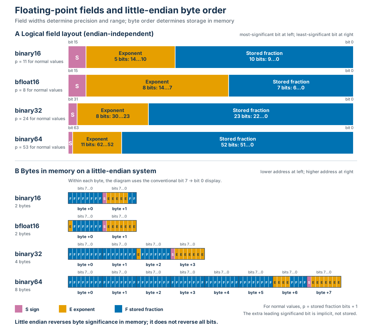
Predict Before Running
- Do binary16 and bfloat16 make the same rounding choices?
- Is spacing constant near \(10^{-6}\), \(1\), and \(10^{16}\)?
- For \(x=2^{53}\), does
x + 1.0changex? - Is
NaN == NaN? - Does
(a + b) + cequala + (b + c)?
Spacing Changes With Scale
| Value | Upward binary64 spacing |
|---|---|
| \(10^{-6}\) | \(2.12\times10^{-22}\) |
| \(1\) | \(2.22\times10^{-16}\) |
| \(2^{53}\) | \(2\) |
| \(10^{16}\) | \(2\) |
- Machine epsilon describes spacing near 1
- It is not a universal comparison tolerance
See The Spacing Change
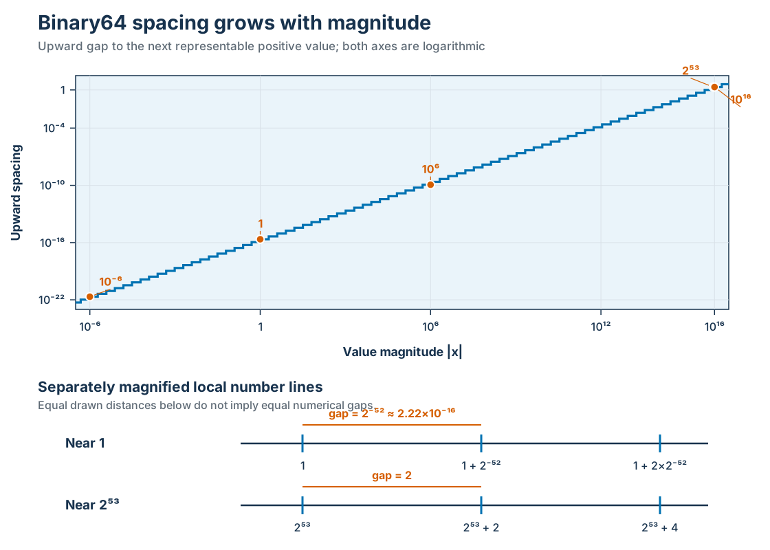
Rounding Is Local
- Form the exact result of one operation
- Select a representable value
- Pass that rounded value to the next operation
x = 2**53
x + 1.0 == x      # True
x + 2.0 == x # FalseNumerical States At The Limits
- Normal: full significand precision
- Subnormal: gradual underflow with reduced precision
- Signed zero: equal values with retained direction
- Infinity: beyond the finite range
NaN: invalid or indeterminate numerical result
Evaluation Order Matters
a = 1e16; b = -1e16; c = 1.0

(a + b) + c  -> 1.0
a + (b + c) -> 0.0- Real-number addition is associative
- Floating-point addition is not generally associative
- Algebraic equivalence does not ensure computational equivalence
Explain The Variance Result
- Centered values: \([-6,-3,3,6]\ \mathrm{ns}\)
- Shortcut intermediates: approximately \(10^{16}\ \mathrm{ns}^2\)
- Local spacing there: \(2\ \mathrm{ns}^2\)
- Exact variance: \(22.5\ \mathrm{ns}^2\)
- Computed shortcut variance: \(22.0\ \mathrm{ns}^2\)
From Explanation To Comparison
- Record the format and rounding assumptions
- Inspect important intermediate scales
- Classify exceptional values explicitly
- Treat evaluation order as part of the computation
- Next question: does the discrepancy matter?
Module 3: Measuring And Comparing Numerical Error
Module Arc
- Qualify the comparison reference
- Match the error measure to the scale
- Treat zero and non-finite values explicitly
- Justify tolerances from requirements
- Match collection summaries to the scientific target
Name The Reference First
- Exact value: error can be stated directly
- High-accuracy result: justify its formulation and convergence
- Benchmark: agreement under documented conditions
- Independent estimate: complementary, not infallible
- Expected range: consistency, not pointwise error
Absolute And Relative Error
\[ E_\mathrm{abs}=|\hat{x}-x_\mathrm{ref}| \]
\[ E_\mathrm{rel}=\frac{|\hat{x}-x_\mathrm{ref}|}{|x_\mathrm{ref}|} \]
- Absolute error retains the quantity’s units
- Relative error is dimensionless
- Relative error is undefined at a zero reference
Predict Across Scales
Requirement:
\[ |\hat{x}-x_\mathrm{ref}| \leq 10^{-5}\ \mathrm{Pa}+10^{-6}|x_\mathrm{ref}| \]
- Reference at zero
- Reference near \(10^{-6}\ \mathrm{Pa}\)
- Reference near \(1\ \mathrm{Pa}\)
- Reference near \(10^6\ \mathrm{Pa}\)
A Mixed Criterion
\[ |\hat{x}-x_\mathrm{ref}| \leq a+r|x_\mathrm{ref}| \]
- \(a\geq0\): absolute tolerance in the quantity’s units
- \(r\geq0\): dimensionless relative tolerance
- Near zero, \(a\) supplies the meaningful floor
- At large scales, the relative term dominates
Three Criteria, Four Decisions
| Case | Absolute only | Relative only | Mixed |
|---|---|---|---|
| Zero | Pass | Undefined | Pass |
| Near zero | Pass | Fail | Pass |
| Order one | Fail | Fail | Fail |
| Large | Fail | Pass | Pass |
A Tolerance Is A Claim
- Name the quantity, units, and reference
- Derive each term from a requirement
- Define zero, boundary,
NaN, and infinity policies - Test intended passes and failures
- Record the rationale before adjusting the threshold
Machine Epsilon Is Not The Policy
- Binary64 epsilon describes spacing near 1
- It has no physical units
- It does not encode input or model limitations
- It does not know the downstream decision
- An unexplained multiplier adds no scientific rationale
Collections Need A Target
- Component-wise: enforce every local requirement
- Maximum error: expose the worst component
- RMS error: describe a typical squared-error scale
- Derived observable: test the quantity driving the conclusion
9 errors of 0.1 Pa, 1 error of 1.0 Pa
maximum = 1.0 Pa, RMS = 0.33 PaFrom Size To Cause
- A passed check supports one bounded comparison claim
- Error, uncertainty, discretization, and variability remain distinct
- A metric describes discrepancy size and structure
- It does not identify why the discrepancy occurred
Module 4: Conditioning And Numerical Stability
Module Arc
- Separate the problem, algorithm, and implementation
- Measure input-to-output sensitivity
- Propagate declared input bounds or uncertainties
- Compare forward and backward error
- Interpret residuals using conditioning
- Match the remedy to the diagnosed cause
Three Different Questions
| Question | Object |
|---|---|
| How sensitive is the answer to input? | Mathematical problem |
| Does the method add avoidable error? | Algorithm |
| Does the code perform that method? | Implementation |
Observe Problem Sensitivity
\[ \kappa_\mathrm{obs}= \frac{\|\Delta x\|/\|x\|} {\|\Delta b\|/\|b\|} \]
- State the norm and scaling
- Perturb inputs independently of the algorithm
- One direction is not the worst-case condition number
Name The Map Before Measuring It
\[ f_\delta:b\mapsto x, \qquad \begin{aligned} x_1+x_2&=b_1,\\ x_1+(1+\delta)x_2&=b_2 \end{aligned} \]
- Input: right-hand side \(b=(b_1,b_2)\)
- Output: exact solution \(x=(x_1,x_2)\)
- Fixed during one perturbation: \(\delta\)
Same Perturbation, Different Sensitivity
\[ b_\delta=(2,2+\delta),\quad x=(1,1) \]
\[ \Delta b=(0,\eta) \quad\Longrightarrow\quad \Delta x=(-\eta/\delta,\eta/\delta) \]
With \(\eta=10^{-16}\):
| \(\delta\) | Relative RHS input | Relative solution output | Amplification |
|---|---|---|---|
| \(1\) | \(3.33\times10^{-17}\) | \(10^{-16}\) | \(3\) |
| \(10^{-12}\) | \(5.00\times10^{-17}\) | \(10^{-4}\) | \(2\times10^{12}\) |
See The Geometry
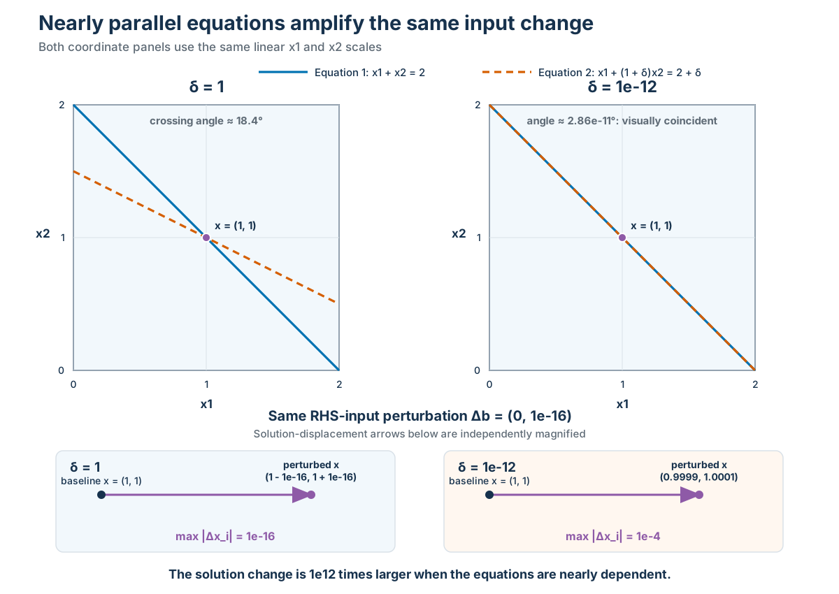
From Sensitivity To Propagation
For \(y=f(x_1,\ldots,x_n)\) and small input changes:
\[ \Delta y\approx\sum_i c_i\Delta x_i, \qquad c_i=\frac{\partial f}{\partial x_i} \]
- \(c_i\) converts input units to output units
- Bounded changes: \(|\Delta y|\lesssim\sum_i|c_i|b_i\)
- Standard uncertainty: \(u_c^2(y)\approx J\Sigma_xJ^\mathsf{T}\)
Same Magnitudes, Different Claims
For \(\rho=m/V\), \(m=100.0\ \mathrm{g}\) and \(V=40.0\ \mathrm{cm^3}\):
| Input interpretation | Propagated result |
|---|---|
| Bounds \(0.2\ \mathrm{g}\), \(0.3\ \mathrm{cm^3}\) | \([2.47643,2.52393]\ \mathrm{g\,cm^{-3}}\) |
| Independent standard uncertainties | \(u_c(\rho)\approx0.0194\ \mathrm{g\,cm^{-3}}\) |
- A deterministic range is not a confidence interval
- Covariance records whether inputs tend to vary together
- Its cross-term can raise or lower propagated variance
First Order Can Fail
For \(Y=X^2\) at nominal \(x=0\):
\[ \left.\frac{dY}{dX}\right|_{x=0}=0 \]
- Linearization predicts zero output uncertainty
- Nonzero plausible inputs still produce positive outputs
- Check with corners, bounds, optimization, or sampled propagation
- Monte Carlo needs a justified joint input distribution
Formal Forward Error
Let \(S(d)\) be the acceptable exact solutions for data \(d\):
\[ e_{\mathrm{fwd}}(\hat{x};d)= \inf_{x\in S(d)} \rho_X(\hat{x},x) \]
For a unique nonzero solution \(x\):
\[ e_{\mathrm{fwd,rel}}= \frac{\|\hat{x}-x\|_X}{\|x\|_X} \]
- Must state the solution or branch, norm, and scaling
Formal Backward Error
Let \(S(d)\) be the exact solutions for data \(d\):
\[ \eta(\hat{x};d)= \inf_{\Delta d\ \mathrm{admissible}} \left\{ \rho_D(d,d+\Delta d): \hat{x}\in S(d+\Delta d) \right\} \]
- Infimum of allowed data changes that make \(\hat{x}\) exact
- Must state structure, norm, and scaling
Backward Stability
- Forward error: is the computed answer close?
- Backward error: is it exact for a nearby input?
- Backward stable: \(\eta(\hat{x};d)\le C u\) for a stated input class
- Ill-conditioning can amplify that perturbation
\[ \text{forward error} \lesssim \kappa\times\text{backward error} \]
Hold The Problem Fixed
Small root of \(x^2-10^8x+1=0\):
\[ \frac{10^8-\sqrt{10^{16}-4}}{2} \quad\text{or}\quad \frac{2}{10^8+\sqrt{10^{16}-4}} \]
- Same polynomial and binary64 format
- Algebraically equivalent algorithms
- 80- and 100-digit reference calculations agree
Compare The Algorithms
| Method | Forward error | Coefficient backward error |
|---|---|---|
| Direct | \(2.55\times10^{-1}\) | \(1.46\times10^{-1}\) |
| Reformulated | \(7.91\times10^{-17}\) | \(3.95\times10^{-17}\) |
- Conditioning is shared by both methods
- Their numerical behaviour is not
- Evidence applies to this tested coefficient set
Residual Is Not Forward Error
For \(A\hat{x}=b-r\):
- Residual: \(r=b-A\hat{x}\)
- RHS backward error: \(\|r\|/\|b\|\)
- Forward error: \(\|\hat{x}-x\|/\|x\|\)
Small Residual, Wrong Answer
Nearly dependent system with \(\delta=10^{-12}\):
| Quantity | Value |
|---|---|
| Exact solution | \((1,1)\) |
| Candidate | \((0,2)\) |
| Relative forward error | \(1\) |
| Relative RHS backward error | \(5\times10^{-13}\) |
Match Evidence To Cause
- High-precision input perturbation → conditioning evidence
- Equivalent algorithm comparison → formulation evidence
- Forward plus backward error → accuracy and nearby-problem evidence
- Known cases and invariants → implementation evidence
- Precision change alone → useful, but not a complete diagnosis
Match Remedy To Cause
- Ill-conditioned problem: improve data, reformulate, or revise the claim
- Unstable algorithm: change formulation, scaling, library, or precision
- Implementation defect: fix the code and add a regression test
- Regularization changes the problem and must be documented
Module 5: Common Numerical Failure Modes
Module Arc
- Diagnose a failed intermediate, not “floating point” in general
- Preserve small increments and low-order contributions
- Keep intermediates inside the usable range
- Match reformulation to cause and validate the result
Carry The Module 4 Questions Forward
- Is the exact problem sensitive?
- Does the algorithm introduce avoidable error?
- Does the implementation perform that algorithm?
- Hold the mathematical input-output map fixed
- Compare against a reference or invariant
Prediction: A Small Increment
For \(x=10^{-16}\), compare
\[ e^x-1 \]
using:
exp(x) - 1expm1(x)- an independently checked decimal reference
Cancellation Result
| Method | Result | Relative error |
|---|---|---|
exp(x) - 1 |
\(0\) | \(1\) |
expm1(x) |
\(1.0\times10^{-16}\) | \(7.09\times10^{-17}\) |
- Reference: \(1.00000000000000005\times10^{-16}\)
- 80- and 100-digit reference calculations agree
Diagnose Cancellation
- Identify the nearby operands and desired difference
- Ask whether operand errors dominate that difference
- Sweep the separation while holding the exact function fixed
- Prefer a validated identity or specialized operation
Examples: expm1, log1p, reformulated quadratic roots
Prediction: One Sum, Five Algorithms
\[ [10^{16},\underbrace{1,\ldots,1}_{10\,000},-10^{16}] \]
- All inputs are exactly representable
- Exact sum: \(10\,000\)
- Which contributions survive each evaluation tree?
Summation Results
| Method | Result | Relative error |
|---|---|---|
| Left to right | \(0\) | \(1\) |
| Magnitude order | \(10\,000\) | \(0\) |
| Pairwise tree | \(9\,998\) | \(2\times10^{-4}\) |
| Neumaier compensation | \(10\,000\) | \(0\) |
math.fsum |
\(10\,000\) | \(0\) |
Sum Conditioning Still Matters
\[ \kappa_{\mathrm{sum}}= \frac{\sum_i |x_i|}{|\sum_i x_i|} \]
- A stable reduction reduces arithmetic error
- A large \(\kappa_{\mathrm{sum}}\) exposes input sensitivity
- No summation method recovers information absent from the data
Choose A Reduction Contract
- Sequential: simple, error can grow with \(n\)
- Pairwise: tree depth near \(\log_2 n\), parallel-friendly
- Compensated: retains discarded low-order information
- Magnitude ordering: sometimes helpful, costs sorting
- Library reduction: prefer documented guarantees
Prediction: A Finite Norm
For \(x=y=10^{308}\):
\[ \sqrt{x^2+y^2} \approx 1.4142\times10^{308} \]
- The final result is representable
- Are the intermediate squares representable?
- Which bound can detect a failed result?
Scale Before Squaring
\[ m=\max(|x|,|y|),\qquad \|(x,y)\|_2=m\sqrt{(x/m)^2+(y/m)^2} \]
| Method | Result |
|---|---|
| Naive squares | \(\infty\) |
| Scaled formula | \(1.4142135623730951\times10^{308}\) |
hypot |
\(1.4142135623730951\times10^{308}\) |
Underflow Depends On Intermediates
\[ 10^{-200}\times10^{-200}\times10^{200}=10^{-200} \]
| Evaluation | Result |
|---|---|
| \((10^{-200}10^{-200})10^{200}\) | \(0\) |
| \(10^{-200}(10^{-200}10^{200})\) | \(10^{-200}\) |
Compare Likelihoods In Log Space
\[ \log\left(\prod_i p_i\right)=\sum_i\log p_i \]
- \(10^{-400}\) and \(10^{-401}\) both become zero in binary64
- Log likelihoods remain finite
- Their difference is \(\log(10)\)
- Keep comparison and normalization in log space
Run The Failure-Mode Lab
- Predict before each execution
- Record the failed intermediate
- Compare with the stated reference or invariant
- Change one scale or order at a time
Match Remedy To Cause
| Failure | Targeted response |
|---|---|
| Nearby subtraction | Identity or specialized function |
| Lost reduction terms | Pairwise or compensation |
| Overflowing powers | Scale first |
| Underflowing product | Rescale, split exponent, or use logs |
| Order dependence | Select and document the tree |
Evidence Has A Scope
- Decimal references are checked at two precisions
- The summation reference is exact
- The norm has a reference and an independent bound
- Examples isolate arithmetic, not measurement uncertainty
- Selected cases do not establish global stability theorems
Module 5 Takeaways
- Find the first intermediate that loses useful information
- Treat summation order as part of the numerical method
- Scale intermediates before they leave the usable range
- Match reformulation to the diagnosed failure
- Validate the change and state its limits
Module 6: Iterative Algorithms And Convergence
Module Arc
- Separate desired error from observable proxies
- Give stopping criteria scales and units
- Detect convergence and recognizable failure
- Find an attainable accuracy floor
- Record why the iteration ended
Error, Residual, And Update
\[ e_k=x_k-x^*,\qquad r_k=f(x_k),\qquad \Delta x_k=x_{k+1}-x_k \]
| Quantity | Question | Observable? |
|---|---|---|
| Error | How far from the desired answer? | Usually no |
| Residual | How well is the equation satisfied? | Usually yes |
| Update | How much did the iterate move? | Yes |
Stopping Is A Claim
\[ \lVert r_k\rVert\le a_r+\rho_r R \]
\[ \lVert\Delta x_k\rVert\le a_x+\rho_x X_k \]
- Name each quantity, norm, unit, and scale
- Keep an absolute floor near zero
- Decide which criteria must hold together
Prediction: One Relative Error, Two Scales
Solve \(x=b\) with a candidate \(x=0.9b\):
| \(b\) | \(|b-x|\) | Relative residual |
|---|---|---|
| \(10^{-12}\) | \(10^{-13}\) | \(0.1\) |
| \(10^{12}\) | \(10^{11}\) | \(0.1\) |
What does an absolute threshold of \(10^{-6}\) report?
A Controlled Relaxation
\[ x_{k+1}=x_k+\omega(b-x_k) \]
For \(x^*=b\):
\[ e_{k+1}=(1-\omega)e_k \]
- \(0<\omega<2\): contraction
- \(\omega=2\): two-cycle
- \(\omega>2\): growing error
Prediction: Classify Four Runs
| Case | \(b\) | \(x_0\) | \(\omega\) |
|---|---|---|---|
| Contracting | \(1\) | \(0\) | \(0.5\) |
| Two-cycle | \(1\) | \(0\) | \(2\) |
| Growing | \(1\) | \(0\) | \(3\) |
| Tiny step | \(2\) | \(1\) | \(10^{-20}\) |
Predict the iterate pattern and termination reason.
Four Runs, Four Reasons
| Case | Iterations | Final residual | Final update | Reason |
|---|---|---|---|---|
| Contracting | 27 | \(7.45\times10^{-9}\) | \(7.45\times10^{-9}\) | converged |
| Two-cycle | 2 | \(1\) | \(-2\) | oscillating |
| Growing | 3 | \(-8\) | \(12\) | diverging |
| Tiny step | 1 | \(1\) | \(0\) | stagnated |
A Zero Update Can Be False Convergence
For \(b=2\), \(x_0=1\), \(\omega=10^{-20}\):
\[ x_1=\operatorname{fl}(1+10^{-20})=1 \]
- Computed update: \(0\)
- Residual: \(1\)
- Update-only decision: accept
- Combined decision:
stagnated
Failure Is A Reportable Result
converged: all required criteria holdstagnated: no computed movement while criteria failoscillating: a declared cycle detector triggersdiverging: a declared growth detector triggersnon_finite: an iterate or diagnostic is NaN or infinitemax_iterations: the budget is exhausted
Prediction: Newton Meets Binary64
\[ x_{k+1}=\frac12\left(x_k+\frac{2}{x_k}\right), \qquad r_k=x_k^2-2 \]
From \(x_0=1\), compare relative tolerances:
- practical: \(10^{-14}\)
- strict: \(10^{-16}\)
Will the stricter request improve the answer?
Same Answer, Different Evidence
| Request | Iterations | Relative residual | Forward error | Reason |
|---|---|---|---|---|
| \(10^{-14}\) | 6 | \(2.22\times10^{-16}\) | \(8.87\times10^{-17}\) | converged |
| \(10^{-16}\) | 6 | \(2.22\times10^{-16}\) | \(8.87\times10^{-17}\) | stagnated |
Both return 1.414213562373095.
Why The Residual Is Informative Here
For the positive root:
\[ x-\sqrt{2}=\frac{x^2-2}{x+\sqrt{2}} \]
- Numerator: the observed residual
- Denominator: well-scaled near the root
- Decimal reference: independent forward-error check
This relationship is problem-specific.
Tolerance Study
| Relative tolerance | Iterations | Forward error | Reason |
|---|---|---|---|
| \(10^{-2}\) | 3 | \(1.50\times10^{-6}\) | converged |
| \(10^{-4}\) | 4 | \(1.13\times10^{-12}\) | converged |
| \(10^{-8}\) | 5 | \(8.87\times10^{-17}\) | converged |
| \(10^{-14}\) | 6 | \(8.87\times10^{-17}\) | converged |
| \(10^{-16}\) | 6 | \(8.87\times10^{-17}\) | stagnated |
Record The Termination Contract
- Problem, method, arithmetic environment
- Initial value and solver parameters
- Residual and update definitions
- Norms, scales, absolute and relative tolerances
- Iteration count and termination reason
- Final residual, update, and selected history
Run The Convergence Activity
- Predict before each run
- Change one relaxation factor
- Compare update-only and combined decisions
- Locate the Newton accuracy floor
Evidence Has A Scope
- Relaxation behaviour is checked against a known recurrence
- Newton forward error uses a 100-digit decimal reference
- A direct identity relates residual and error for this root
- Cycle and growth detectors are intentionally simple
- No model, input, or discretization has been validated
Module 6 Takeaways
- Error, residual, and update answer different questions
- Give every tolerance a quantity, unit, norm, and scale
- Reject small-update false convergence with independent evidence
- Report failure reasons and exhausted budgets explicitly
- Use tolerance studies to find attainable accuracy
Module 7: Validating Scientific Computations
Module Arc
- Separate implementation, solution, and model claims
- Match each claim to evidence that can challenge it
- Test exact cases, properties, and refinement rates
- Prefer comparison methods that fail differently
- Preserve observations and limitations as a portfolio
Three Questions, Three Evidence Needs
- Code verification: Is the method implemented correctly?
- Solution verification: Is numerical error controlled here?
- Model validation: Does the model represent the intended system?
Analytic tests cannot replace experimental evidence.
Start With The Claim
| Claim | Candidate evidence |
|---|---|
| Method is implemented | Exact case or method property |
| Approximation is controlled | Refinement trend and error estimate |
| Result is not method-specific | Independent algorithm |
| Model represents reality | Experimental or observational data |
References Have Different Authority
- Exact analytic value
- Manufactured or limiting case
- Checked high-precision calculation
- Published benchmark with matching conditions
- Experimental data with uncertainty
State what each reference shares with the candidate.
Properties Reject Impossible Results
- Conservation and balance
- Positivity and bounds
- Symmetry and monotonicity
- Dimensional consistency
- Exactness for a class of inputs
Necessary does not mean sufficient.
Validation Problem: One Integral
\[ I=\int_0^1 e^x\,\mathrm{d}x=e-1 \]
- Positive, increasing, and convex integrand
- Exact analytic reference
- Predicted quadrature orders
- Independent factorial-series formulation
Two Claimed Trapezoidal Candidates
\[ T_n=h\left[\frac{f(0)}2+\sum_{i=1}^{n-1}f(ih)+\frac{f(1)}2\right] \]
\[ S_n=h\sum_{i=0}^{n-1}f(ih) \]
Which reference input distinguishes them?
Prediction: Constant Exactness
For \(f(x)=1\) on \([0,1]\) with \(n=8\):
- Exact integral: \(1\)
- What does \(T_8\) return?
- What does \(S_8\) return?
- Which endpoint-weight claim is tested?
One Pass Is Not A Portfolio
| Candidate | Constant result | Error |
|---|---|---|
| Intended trapezoidal | \(1\) | \(0\) |
| Suspicious candidate | \(1\) | \(0\) |
The test does not exercise endpoint weights.
Prediction: Affine Exactness
For \(f(x)=x\) on \([0,1]\):
\[ \int_0^1x\,\mathrm{d}x=\frac12 \]
The trapezoidal rule must integrate every affine function exactly.
The Stronger Case Diagnoses The Method
| Candidate | Result at \(n=8\) | Error |
|---|---|---|
| Intended trapezoidal | \(0.5\) | \(0\) |
| Suspicious candidate | \(0.4375\) | \(0.0625\) |
The suspicious code implements a first-order left rule.
A Broad Bound Still Passes
For positive, increasing \(e^x\):
\[ 1\le Q_n\le e \]
- Trapezoidal: passes
- Midpoint: passes
- Suspicious left rule: passes
Plausibility is useful but incomplete.
Prediction: Refinement Rate
If \(E(h)\approx Ch^p\), then
\[ p_{\mathrm{obs}}=log_2\frac{|E_n|}{|E_{2n}|} \]
- Trapezoidal prediction: \(p=2\)
- Midpoint prediction: \(p=2\)
- Left-endpoint prediction: \(p=1\)
Refinement Identifies The Contract
| Method | Error, \(n=8\) | Error, \(n=64\) | Observed \(p\) |
|---|---|---|---|
| Trapezoidal | \(2.24\times10^{-3}\) | \(3.50\times10^{-5}\) | \(2.00\) |
| Midpoint | \(1.12\times10^{-3}\) | \(1.75\times10^{-5}\) | \(2.00\) |
| Suspicious | \(1.05\times10^{-1}\) | \(1.34\times10^{-2}\) | \(1.00\) |
Convexity Brackets The Integral
For convex \(e^x\):
\[ M_n\le I\le T_n \]
At \(n=8\):
\[ 1.717163664995687<I<1.720518592164302 \]
How Independent Is Agreement?
Midpoint and trapezoidal rules differ in:
- sample locations;
- leading-error signs;
- lower versus upper convexity bounds.
They still share the integrand, interval, language, and loop structure.
A Different Calculation: Exact Series
\[ e-1=\sum_{k=1}^{\infty}\frac1{k!} \]
For exact rational \(P_N\):
\[ 0<(e-1)-P_N\le \frac1{(N+1)!}\frac{N+2}{N+1} \]
Check High Precision, Too
- Evaluate the analytic expression at 80 and 100 digits
- Check that the reference digits stabilize
- Preserve input information before raising precision
- Add a bound or different formulation
More digits do not establish authority by themselves.
Run The Validation Activity
- Predict before each check
- Add one refinement level
- Compare claims with observations
- Retain failed and successful evidence
Keep Claims And Limitations Together
| Claim | Observation | Scope |
|---|---|---|
| Constant case works | Both return \(1\) | Weights untested |
| Candidate is trapezoidal | Affine case fails | Claim rejected |
| Error is controlled | Expected order observed | Tested grids only |
| Model represents reality | No observations | Not established |
Module 7 Takeaways
- Separate code, solution, and model claims
- Choose evidence that can challenge each claim
- Predict properties and rates before measuring them
- Prefer methods with different failure modes
- Check reference calculations and retain limitations
Module 8: Reproducibility Across Computing Environments
Module Arc
- Define the agreement required for the scientific use
- Identify how an environment change alters arithmetic
- Compare harmless low-bit variation with a changed conclusion
- Treat parallel partitions and precision as algorithm choices
- Preserve the tested matrix, observations, and limitations
Reproducibility Is A Claim
Name all three:
- Allowed change: compiler, library, hardware, order, precision, seed
- Required agreement: bits, tolerance, distribution, conclusion
- Intended use: debugging, restart, estimate, scientific decision
Different Claims Need Different Evidence
| Level | Required evidence |
|---|---|
| Bitwise identity | Exact serialized comparison |
| Numerical agreement | Justified metric and tolerance |
| Statistical equivalence | Replicates, uncertainty, effect size |
| Same conclusion | Stable decision margin |
Choose The Weakest Sufficient Contract
- Exact restart may require identical state
- Deterministic solvers may allow bounded low-order variation
- Ensembles usually require distributional agreement
- Threshold decisions require a stable margin
Do not weaken a scientifically necessary contract after it fails.
Why Arithmetic Changes
- Reassociation and fused operations
- Math-library algorithms
- Vector width and instruction selection
- Thread or process reduction trees
- Storage and accumulator precision
Change One Factor At A Time
| Hold fixed | Change | Record |
|---|---|---|
| Source and input hash | Reduction order | Bits, error, decision |
| Algorithm and tolerance | Thread count | Partition and partials |
| Quantity and units | Precision | Non-finite states and margin |
| Validation reference | Toolchain | Compiler, flags, libraries |
A Changed Bit Is Not Automatically A Defect
- First confirm inputs, algorithm, and termination are the same
- Classify the arithmetic mechanism
- Apply the predeclared numerical criterion
- Check whether the scientific conclusion survives
- Retain the tested environment scope
Case 1: Positive Calibration Corrections
\[ b_k=\frac1k\ \mathrm{J},\qquad k=1,\ldots,10{,}000 \]
- Stored-input reference: \(9.787606036044382\ \mathrm{J}\)
- Numerical budget: \(10^{-10}\ \mathrm{J}\)
- Decision: does the total exceed \(9.5\ \mathrm{J}\)?
Prediction: Reverse The Order
For positive binary64 terms, will reversal change:
- the hexadecimal output?
- the pass/fail result at \(10^{-10}\ \mathrm{J}\)?
- the above-\(9.5\ \mathrm{J}\) conclusion?
Different Bits, Adequate Result
| Order | Total (J) | Absolute error (J) |
|---|---|---|
| Original | \(9.787606036044348\) | \(3.40\times10^{-14}\) |
| Reverse | \(9.787606036044386\) | \(3.29\times10^{-15}\) |
| Increasing magnitude | \(9.787606036044386\) | \(3.29\times10^{-15}\) |
All pass the budget and remain above \(9.5\ \mathrm{J}\).
Do Not Overstate The Pass
Supported:
- Three tested orders satisfy the declared numerical budget
- The tested conclusion has a large margin
Not established:
- Every compiler, library, processor, or future input behaves likewise
Case 2: Cancellation-Sensitive Energy Ledger
- Source: \(+2^{53}\ \mathrm{J}\)
- Sink: \(-2^{53}\ \mathrm{J}\)
- 4,096 contributions: \(+0.5\ \mathrm{J}\) each
- Exact stored-input total: \(2048\ \mathrm{J}\)
Balance is acceptable only when \(|E|\le100\ \mathrm{J}\).
Prediction: Where Do The Small Terms Go?
At \(2^{53}\), binary64 spacing is \(2\ \mathrm{J}\).
Compare:
- source → small terms → sink
- source → sink → small terms
- small terms → source → sink
One Order Reverses The Conclusion
| Order | Net energy (J) | Classification |
|---|---|---|
| Source, smalls, sink | \(0\) | Acceptable—wrong |
| Source, sink, smalls | \(2048\) | Material imbalance |
| Smalls, source, sink | \(2048\) | Material imbalance |
One-percent numerical budget: \(|E-2048|\le1\ \mathrm{J}\).
Sensitivity Predicts Risk
\[ \kappa_{\mathrm{sum}}= \frac{\sum_i|x_i|}{|\sum_i x_i|} \approx8.80\times10^{12} \]
- Large contributions nearly cancel
- The desired net is small relative to absolute input mass
- Order, precision, and input uncertainty need scrutiny
Parallel Reduction = Numerical Algorithm
- Partition the global data
- Reduce within each partition
- Combine partial results in a tree
Thread count, rank count, and scheduling can change both groupings.
Partition Count Changes The Result
| Contiguous chunks | Net energy (J) | Error (J) |
|---|---|---|
| 1 | \(0\) | \(2048\) |
| 2 | \(1024\) | \(1024\) |
| 4 | \(1536\) | \(512\) |
| 8 | \(1792\) | \(256\) |
| 16 | \(1920\) | \(128\) |
The selected trend is not guaranteed to continue.
Deterministic Does Not Mean Accurate
- Fixed tree: repeatable grouping, possibly repeatable error
- Pairwise or compensated sum: usually more accurate, not necessarily bitwise
- Long or exact accumulator: stronger result, additional cost
- Tolerance check: useful only when tied to the scientific requirement
Accumulator Precision Is Part Of The Contract
“16-bit support” does not identify the arithmetic:
| Stage | Record |
|---|---|
| Input and storage | binary16, bfloat16, binary32, … |
| Operations | product, sum, fused or library-kernel format |
| Accumulation | partial-sum format and rounding points |
| Output | conversion, format, and rounding rule |
The Tested Accumulator Policy
| Order | Binary64 (J) | Binary32-rounded (J) |
|---|---|---|
| Source, smalls, sink | \(0\) | \(0\) |
| Source, sink, smalls | \(2048\) | \(2048\) |
| Smalls, source, sink | \(2048\) | \(0\) |
Record storage, product, and accumulator precision separately.
Compiler And Library Controls Have Scope
- Strict modes can restrict reassociation or contraction
- Library versions can change transcendental or reduction algorithms
- A fixed flag name need not mean the same thing across toolchains
- Serialization and exceptional values can break bitwise contracts
Verify executable behaviour; do not trust a label alone.
Seeds Do Not Define Statistical Equivalence
When exact sequences matter, record:
- generator family and algorithm;
- library version and seed;
- stream mapping to threads, ranks, or tasks.
When distributions matter, compare replicated statistical evidence.
Run The Reproducibility Activity
- Predict three agreement levels separately
- Change one partition count
- Inspect result bits, error, and decision margin
- Build a claim-environment-observation record
Keep The Reproducibility Record With The Result
- Source revision, build recipe, and dirty-state status
- Input identity, units, range, preprocessing, and fingerprint
- Algorithm, precision, tolerance, and termination reason
- Libraries, hardware, threads/ranks, decomposition, and seeds
- Observed difference, classification, and limitations
Interpret The Tested Matrix
| Observation | Report |
|---|---|
| Bits differ; tolerance passes | Numerically reproducible, if bits were not required |
| Tolerance fails; conclusion stays | Conclusion survived; accuracy contract failed |
| Conclusion changes | Claim is not reproducible over this change |
| All tested bits match | Bitwise identity over the tested matrix only |
Module 8 Takeaways
- Define allowed changes and required agreement before running
- Diagnose mechanisms, not vague machine labels
- Treat reduction trees and precision as algorithm choices
- Check numerical evidence and the scientific decision separately
- Report the tested matrix and what remains unverified
Module 9: Communicating Numerical Reliability
Module Arc
- Lead with the quantity, units, and intended decision
- Keep error, uncertainty, variability, and model limits distinct
- Match displayed digits to the supported scale
- Compress evidence without replacing it
- Write a qualified claim that remains useful
A Report Is A Compact Argument
Connect:
- Claim — what is being asserted?
- Evidence — what can challenge it?
- Margin — how close is the requirement?
- Scope — where does the conclusion apply?
- Limitation — what could still change it?
Start With The Decision-Facing Quantity
- Quantity and units
- Input range and operating regime
- Assumed model
- Decision or downstream use
- Accuracy scale that could change the decision
“Eight iterations” is evidence—not the scientific claim.
Four Layers, Four Questions
| Layer | Question |
|---|---|
| Result | What quantity was obtained? |
| Numerical evidence | Why is the computation adequate? |
| Interpretation | What decision follows? |
| Limitation | What remains unestablished? |
Reporting Case: Heating Energy
\[ P(t)=P_0\exp(t/\tau),\qquad 0\le t\le\tau \]
\[ E=P_0\tau\int_0^1e^x\,\mathrm{d}x \]
- \(P_0\) in kilowatts
- \(\tau=1.00\ \mathrm{h}\)
- \(E\) in kilowatt-hours
Declare Inputs And Requirements
| Item | Value |
|---|---|
| Nominal power | \(12.0\ \mathrm{kW}\) |
| Admissible power | \([11.9,12.1]\ \mathrm{kW}\) |
| Decision threshold | \(20.0\ \mathrm{kWh}\) |
| Numerical budget | \(0.01\ \mathrm{kWh}\) |
| Candidate | 64-panel trapezoidal rule |
Prediction: What Must The Report Prove?
Before calculating, identify evidence for:
- numerical adequacy at 64 panels;
- robustness over the power range;
- harmless tested environment variation;
- physical validity of the exponential model.
Which item cannot be established here?
Quantify Numerical Error
Analytic model reference:
\[ E_{\mathrm{ref}}=20.6193819415085428\ldots\ \mathrm{kWh} \]
64-panel result:
\[ E_{T,64}=20.619801442201130\ \mathrm{kWh} \]
Absolute error: \(4.20\times10^{-4}\ \mathrm{kWh}\)
Refinement Supports The Method Claim
| Panels | Error (kWh) | Observed order |
|---|---|---|
| 8 | \(2.68\times10^{-2}\) | — |
| 16 | \(6.71\times10^{-3}\) | \(2.00\) |
| 32 | \(1.68\times10^{-3}\) | \(2.00\) |
| 64 | \(4.20\times10^{-4}\) | \(2.00\) |
Error Is Not A Generic Uncertainty
Keep separate:
- Floating-point and discretization error
- Iteration error and stopping evidence
- Input range or measurement uncertainty
- Model discrepancy
- Stochastic and environment variability
Shared units do not justify adding them.
Numerical Bounds At Nominal Input
Convexity gives
\[ 20.619172191802360 \le E \le 20.619801442201130\ \mathrm{kWh}. \]
Bracket width:
\[ 6.29\times10^{-4}\ \mathrm{kWh} \]
Propagate The Declared Input Range
Monotonicity gives the deterministic envelope
\[ 20.4473\le E\le20.7916\ \mathrm{kWh}. \]
- Lower endpoint exceeds \(20.0\ \mathrm{kWh}\)
- Conservative margin is about \(0.45\ \mathrm{kWh}\)
- No probability coverage is implied
Prediction: Which Digits Belong In The Headline?
Candidate output:
20.619801442201130 kWhInput-range envelope width:
about 0.34 kWhWhat should a decision-facing report display?
Report The Supported Scale
- Nominal result: \(20.62\ \mathrm{kWh}\)
- Deterministic envelope: \([20.45,20.79]\ \mathrm{kWh}\)
- Threshold: \(20.0\ \mathrm{kWh}\)
- Conservative margin: \(0.45\ \mathrm{kWh}\)
Preserve full values in the evidence artifact.
A Complete Tolerance Sentence
Include:
- quantity and units;
- reference;
- metric;
- threshold and rationale;
- observation and outcome.
Compress Evidence, Retain Scope
| Claim | Compact evidence | Limitation |
|---|---|---|
| Numerical method adequate | Error passes; order two | Smooth model case |
| Input range preserves decision | Envelope above threshold | \(P_0\) only |
| Tested order variation harmless | Low-bit spread; same decision | One runtime |
| Model represents reality | No observations | Not established |
Report Environment Variation At The Tested Level
| Reduction | Energy (kWh) |
|---|---|
| Forward serial | \(20.619801442201130\) |
| Reverse serial | \(20.619801442201123\) |
| Accurate sum | \(20.619801442201119\) |
- Bits differ
- Spread is about \(1.1\times10^{-14}\ \mathrm{kWh}\)
- Budget and conclusion pass
Failed Checks Belong In The Result
- Non-finite output is a categorical failure
- Different termination reasons need explanation
- An unevaluated regime is not a passing regime
- A failed numerical criterion cannot be hidden by an unchanged classification
Do not summarize only successful rows.
Reliability Statement Structure
- Claim and scope
- Rounded result, range, and decision margin
- Strongest numerical evidence
- Tested variability
- Assumptions, failures, and limitations
Weak Pattern: Overclaim
The system delivers exactly \(20.619801442201130\ \mathrm{kWh}\) and safely meets the requirement.
Problems:
- model and inputs treated as exact;
- unsupported digits;
- no evidence or tested scope.
Weak Pattern: Verdict Or Data Dump
The result was validated and is reproducible.
n=8: 20.6462; n=16: 20.6261; n=32: 20.6211; n=64: 20.6198.
Neither statement connects evidence to a requirement.
Qualified Statement: Claim And Result
Under the exponential power model with \(P_0\in[11.9,12.1]\ \mathrm{kW}\), accumulated energy is \([20.45,20.79]\ \mathrm{kWh}\); the nominal result is \(20.62\ \mathrm{kWh}\).
The lower bound remains \(0.45\ \mathrm{kWh}\) above the requirement.
Qualified Statement: Evidence And Limits
Absolute error is \(4.20\times10^{-4}\ \mathrm{kWh}\) against the analytic reference, refinement is second order, and tested reduction orders preserve the decision.
Not established:
- physical validity of the exponential model;
- probability for the input range;
- duration uncertainty or untested platforms.
Layer The Communication Artifact
- Headline result and qualification
- Compact reliability statement
- Evidence table and failed checks
- Source, inputs, configuration, environment, complete outputs
Every layer must support the same claim.
Run The Reporting Activity
- Build the evidence record
- Diagnose weak statements
- Inspect full versus displayed precision
- Revise the statement for a chosen audience
Exercise: Change The Audience, Not The Evidence
Rewrite for:
- a two-sentence paper result;
- a numerical code review;
- an operations threshold decision.
Retain units, scope, evidence, margin, and a consequential limitation.
Module 9 Takeaways
- Lead with the conditional scientific claim
- Keep error and uncertainty sources distinct
- Report evidence, tolerance rationale, and margin together
- Round for communication; retain full evidence precision
- Make failures and limitations visible
- Link concise prose to reproducible artifacts
Module 10: Capstone Investigation
Module Arc
- State the decision before changing the code
- Reproduce the precision-dependent result
- Distinguish residual, forward error, and sensitivity
- Improve arithmetic and decision logic separately
- Validate with complementary evidence
- Report what remains indeterminate
The Stable Total And The Unstable Split
Two compounds, two nearly indistinguishable sensor responses:
\[ y_1=c_A+c_B, \qquad y_2=c_A+(1+\delta)c_B. \]
- \(c_A,c_B\) in \(\mathrm{mg/L}\)
- \(y_1,y_2\) in normalized response units
- \(\delta\) measures sensor separation
The Declared Case
| Item | Value |
|---|---|
| \(y_1\) | \(1.0000000\) response units |
| \(y_2\) | \(1.0000004\) response units |
| \(\delta\) | \(10^{-6}\) |
| Bound on each reading | \(\pm5\times10^{-8}\) response units |
| Decision | \(c_A>0.61\ \mathrm{mg/L}\) |
| Required accuracy | \(0.01\ \mathrm{mg/L}\) |
Prediction: What Could Reverse The Decision?
Consider:
- an implementation defect;
- inadequate arithmetic precision;
- sensitivity of the inverse problem;
- admissible variation in the readings;
- an invalid physical response model.
What evidence would distinguish them?
Start The Capstone
Record:
- concentrations and decision;
- residual quantity and units;
- stored precision;
- required accuracy and its units.
The Suspicious Baseline
c_A: 0.625000000 mg/L
c_B: 0.375000000 mg/L
decision: yes
residual infinity norm: 2.500e-08 response units- Positive concentrations
- Total equals \(1\ \mathrm{mg/L}\)
- Small response residual
- Plausible decision
Is the result accurate enough?
Checkpoint 1: Do Not Rewrite Yet
Write down:
- the exact scientific claim;
- the reference you need;
- the error metric you will use;
- one controlled variation;
- one conclusion-changing limitation.
Residual Is Not Forward Error
Response residual:
\[ \lVert A\widehat{c}-y\rVert_\infty \quad\text{in response units} \]
Required component error:
\[ |\widehat{c}_A-c_{A,\mathrm{ref}}| \quad\text{in }\mathrm{mg/L} \]
A bare comparison with 0.01 has no meaning.
Establish A Nominal Reference
\[ c_B=\frac{y_2-y_1}{\delta}, \qquad c_A=y_1-c_B. \]
For the declared decimal inputs:
\[ (c_A,c_B)=(0.6,0.4)\ \mathrm{mg/L}. \]
What does this reference establish?
Precision Changes The Nominal Decision
| Arithmetic | \(c_A\) (mg/L) | Decision |
|---|---|---|
| Binary32 | \(0.625\) | yes |
| Binary64 | \(0.5999999999885\) | no |
| Exact-decimal reference | \(0.6\) | no |
- Binary32 error: \(0.025\ \mathrm{mg/L}\)
- Required accuracy: \(0.01\ \mathrm{mg/L}\)
- Binary64 error: \(1.15\times10^{-11}\ \mathrm{mg/L}\)
Why Is The Split Sensitive?
\[ A= \begin{bmatrix} 1&1\\ 1&1+\delta \end{bmatrix} \]
- \(\delta=0\): identical rows, no unique split
- Small \(\delta\): solvable but sensitive
- At \(\delta=10^{-6}\):
\[ \kappa_2(A)\approx4.00\times10^6 \]
Avoid A Diagnostic Cancellation
For \(A^\mathsf{T}A\):
\[ \operatorname{trace}=4+2\delta+\delta^2, \qquad \det=\delta^2. \]
Compute \(\lambda_{\max}\) directly, then use
\[ \kappa_2(A)=\frac{\lambda_{\max}}{|\delta|}. \]
Do not form the small eigenvalue by subtracting near-equal values.
Controlled Variation: Separate The Sensors
Keep \((c_A,c_B)=(0.6,0.4)\ \mathrm{mg/L}\) known.
| \(\delta\) | \(\kappa_2(A)\) | Binary32 \(c_A\) error |
|---|---|---|
| \(10^{-1}\) | \(4.21\times10^1\) | \(5.01\times10^{-7}\) |
| \(10^{-2}\) | \(4.02\times10^2\) | \(4.79\times10^{-6}\) |
| \(10^{-4}\) | \(4.00\times10^4\) | \(4.77\times10^{-4}\) |
| \(10^{-6}\) | \(4.00\times10^6\) | \(2.50\times10^{-2}\) |
A Revealing Edge Case
At \(\delta=10^{-8}\) in binary32:
sensor separation is zero after binary32 storage- Both response coefficients store as one
- The components are not distinguishable on this path
- Explicit failure is better than a plausible estimate
Checkpoint 2: Which Cause Is Dominant?
Evidence so far:
- Binary32 fails the nominal accuracy requirement
- Binary64 agrees with the nominal reference
- Error grows as sensor separation shrinks
- The well-separated control succeeds
What remains untested before the scientific decision?
Propagate The Reading Bounds
Each reading varies independently by \(\pm5\times10^{-8}\) response units.
- Fixed nonzero \(\delta\)
- Linear mapping from readings to concentrations
- Rectangular input range
- Extrema occur at the four corners
What range should the decision cover?
The Stable Total And The Unstable Split
| Quantity | Deterministic range (mg/L) |
|---|---|
| \(c_A\) | \([0.49999995,0.70000005]\) |
| \(c_B\) | \([0.30,0.50]\) |
| \(c_A+c_B\) | \([0.99999995,1.00000005]\) |
- Component interval crosses \(0.61\ \mathrm{mg/L}\)
- Total remains tightly bounded by \(y_1\)
The Supported Decision
For the strict threshold:
yes: every admissible \(c_A>0.61\ \mathrm{mg/L}\)no: every admissible \(c_A\le0.61\ \mathrm{mg/L}\)indeterminate: the interval crosses the threshold
This case is indeterminate.
Improve One Factor At A Time
| Change | Improvement | Remaining limitation |
|---|---|---|
| Retain binary64 | Nominal arithmetic passes | Input sensitivity |
| Use interval decision | Prevents overclaim | Range remains wide |
| Report total separately | Preserves robust result | Split unresolved |
Higher precision cannot create missing measurement information.
Complementary Validation Portfolio
- Exact-decimal nominal reference
- Binary64 forward-error comparison
- Well-separated synthetic control
- Condition-number trend
- Four-corner input envelope
- Total-concentration invariant
Which checks share the same model assumption?
Run The Completion Checks
- Tests check implementation and evidence structure
- Inspect quantities, units, scope, and limitations
- Passing tests are not scientific approval
Reliability Statement: Result And Evidence
Under the declared linear sensor model, binary64 gives \(c_A=0.600\ \mathrm{mg/L}\) and agrees with the exact-decimal nominal reference to \(1.15\times10^{-11}\ \mathrm{mg/L}\), below the predeclared \(0.01\ \mathrm{mg/L}\) accuracy requirement.
- Binary32 \(c_A\) error: \(0.025\ \mathrm{mg/L}\), which exceeds the requirement
- Nominal decision changes from
noin binary64 toyesin binary32 - \(\kappa_2(A)\approx4.00\times10^6\)
The input-bound consequence follows on the next slide.
Reliability Statement: Decision And Limits
The component interval crosses \(0.61\ \mathrm{mg/L}\), so the supported decision is indeterminate. The total remains in \([0.99999995,1.00000005]\ \mathrm{mg/L}\).
\(c_A\in[0.50,0.70]\ \mathrm{mg/L}\) over the deterministic reading bounds.
Not established:
- physical validity of the linear calibration;
- probability for the reading bounds;
- behaviour on untested precision or hardware paths.
What Would Resolve The Question?
- A sensor with more distinct response coefficients
- A third independently informative measurement
- Tighter justified reading bounds
- Physical calibration and validation over the intended regime
Regularization adds an assumption; it does not recover absent information.
Capstone Completion Criteria
- Suspicious result reproduced and quantified
- Reference scope stated correctly
- Conditioning diagnosis supported by a control
- Arithmetic and input sensitivity separated
- Two or more complementary checks recorded
- Decision covers the complete declared range
- Qualified reliability statement completed
Module 10 Takeaways
- Start from the scientific claim and accuracy requirement
- Treat residuals as diagnostics, not automatic error bounds
- Change one explanatory factor at a time
- Separate arithmetic adequacy from problem identifiability
- Preserve robust quantities and explicit failure states
- Make the conclusion no stronger than the evidence
Wrap Up
The Reliability Workflow
- Define the claim and required accuracy
- Measure the discrepancy
- Separate conditioning, algorithm, and implementation
- Gather independent validation evidence
- Test relevant environment changes
- Report assumptions and limitations
Habits To Keep
- Predict before computing
- Compare against more than one kind of evidence
- Treat tolerances as scientific requirements
- Record termination reasons and environments
- Report fewer digits and stronger evidence