Module 2: Understanding Floating-Point Arithmetic
Motivation
In Module 1, two algebraically equivalent variance formulas produced different answers. The programs ran successfully, the inputs were the same, and both results looked plausible. An exact reference and an invariant identified the defensible result, but they did not explain the discrepancy.
The missing idea is that a computer does not perform arithmetic over all real numbers. A floating-point format stores a finite set of values, and most input conversions and arithmetic operations must choose a representable result. Those choices are systematic rather than random, so we can reason about when they matter.
Learning outcomes
After this module, you should be able to:
- explain sign, significand, exponent, and finite precision conceptually;
- compare how common binary16, bfloat16, binary32, and binary64 formats trade significand precision against exponent range;
- use the spacing between representable values to predict when information can be lost;
- explain why rounding occurs during a sequence of operations, not only when a result is printed;
- recognize normal numbers, subnormal numbers, signed zero, infinity, and
NaNas distinct numerical states; - explain the causes of overflow and underflow;
- demonstrate why algebraically equivalent expressions can compute differently.
Connection to Module 1
Module 1 introduced a workflow for investigating suspicious results. Its variance experiment held the exact inputs and scientific decision fixed, then used a reference calculation and shift invariance as evidence. This module supplies the arithmetic model needed to explain the observed behaviour.
We will not yet decide how large an acceptable discrepancy should be. That requires scale-aware error measures and a scientific accuracy requirement, which belong to Module 3.
A finite model of real numbers
A nonzero normal floating-point number can be described conceptually as
\[ x = (-1)^s \times m \times b^e, \]
where:
- \(s\) determines the sign;
- \(m\) is the significand, which carries the significant digits;
- \(b\) is the base, also called the radix, usually 2 for scientific-computing hardware;
- \(e\) is the exponent, which scales the value by a power of the base.
The significand determines the available precision: how much detail can be retained at a particular scale. The exponent determines much of the range: how small or large a magnitude can be represented. Precision and range are different resources; a format can cover enormous magnitudes without keeping every integer or fraction within that range.
The examples in this course use Python’s float in the published course environment. It is an IEEE 754 binary64 value with 53 bits of significand precision for normal numbers. One bit records the sign, an exponent field selects the scale, and a fraction field records the significant binary digits. The exact bit layout is useful for some systems work, but it is not necessary for the reasoning in this course.
The same model supports different format trade-offs
Scientific software does not always use binary64. Binary32 is common when memory capacity, data movement, or arithmetic throughput matter, provided that the resulting accuracy is adequate. Accelerators and some CPUs also support 16-bit formats. The phrase “16-bit floating point” is incomplete because two important formats allocate those bits differently.
The table compares properties relevant to numerical reasoning. Significand precision includes the implicit leading bit of a normal value; it is therefore one greater than the stored fraction-field width.
| Format | Significand precision | Exponent bits | Gap above 1 | Positive normal range |
|---|---|---|---|---|
| binary16 | 11 bits | 5 | \(2^{-10}\approx9.77\times10^{-4}\) | approximately \(6.10\times10^{-5}\) to \(6.55\times10^4\) |
| bfloat16 | 8 bits | 8 | \(2^{-7}=7.8125\times10^{-3}\) | approximately \(1.18\times10^{-38}\) to \(3.39\times10^{38}\) |
| binary32 | 24 bits | 8 | \(2^{-23}\approx1.19\times10^{-7}\) | approximately \(1.18\times10^{-38}\) to \(3.40\times10^{38}\) |
| binary64 | 53 bits | 11 | \(2^{-52}\approx2.22\times10^{-16}\) | approximately \(2.23\times10^{-308}\) to \(1.80\times10^{308}\) |
Binary16, binary32, and binary64 are IEEE 754 binary interchange formats. Bfloat16 is a different 16-bit layout, not another name for binary16. It keeps the exponent width of binary32, and therefore approximately its normal range, but retains only eight bits of significand precision. Binary16 retains more detail near one but has a much smaller exponent range.
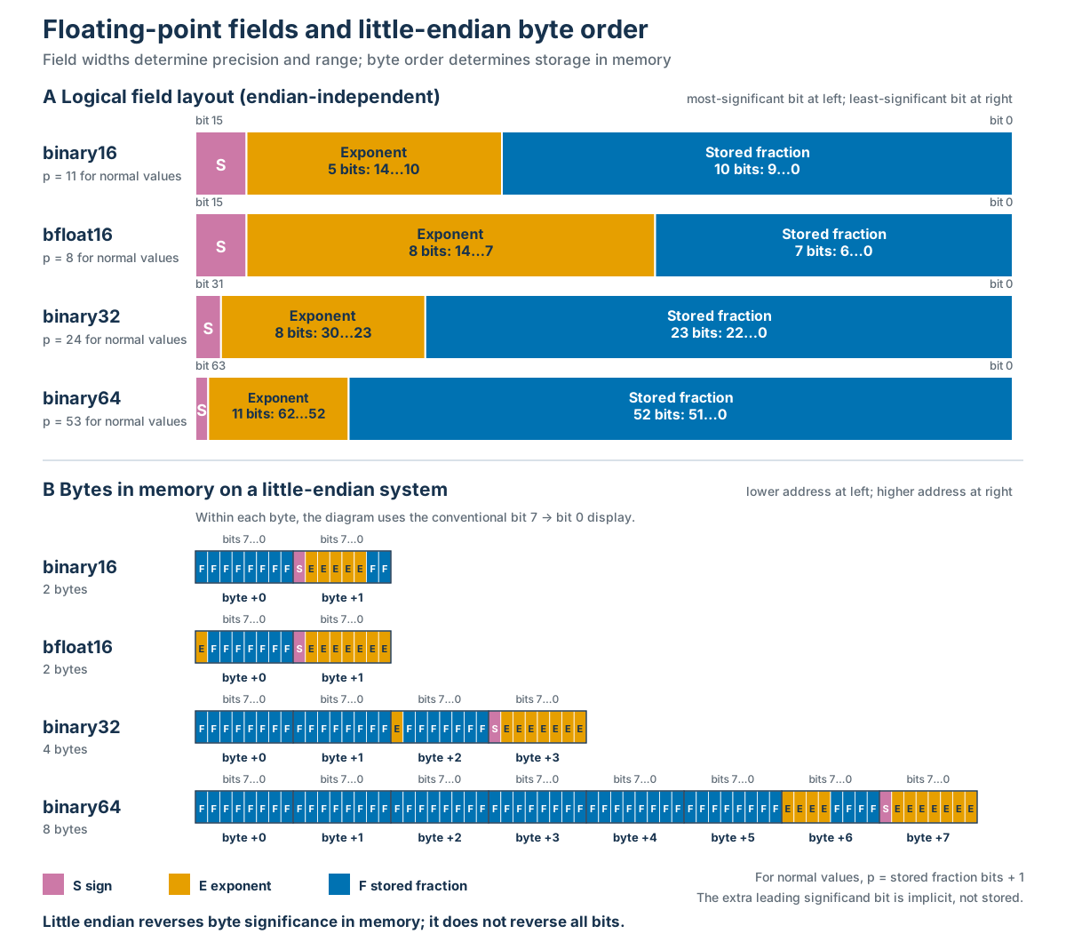
The upper panel is the logical representation, conventionally written from the most-significant bit to the least-significant bit. This field order does not depend on endianness. The lower panel shows how the same bits occupy bytes in increasing memory-address order on a little-endian system: the least-significant byte is stored first. Bits within each byte are still drawn in the conventional bit-7-to-bit-0 direction. Little endian therefore changes byte order; it does not reverse the complete string of bits.
The blue field contains the stored fraction, not the complete significand. For a normal value the leading significand bit is implicit, which is why the precision \(p\) in the table and figure is one greater than the stored fraction width. Subnormal values do not have that implicit leading one, and exponent patterns at the extremes encode zeros, infinities, and NaNs rather than ordinary scaled significands.
Two probes expose the trade-off:
- Near one, binary16 can distinguish
1.001from1, whereas bfloat16 rounds1.001to1under round-to-nearest, ties-to-even. - The value \(10^{-20}\) is far below even the binary16 subnormal range and rounds to zero there. It lies within the normal range of bfloat16, binary32, and binary64.
Likewise, every consecutive integer is representable through \(2^p\), where \(p\) is the significand precision. At that threshold, adding one can already round back to the original value: \(2^8\) for bfloat16, \(2^{11}\) for binary16, \(2^{24}\) for binary32, and \(2^{53}\) for binary64. Some larger integers remain representable, but not every integer does.
These observations do not rank one format as universally best. A narrower format can reduce storage, data movement, and sometimes runtime or energy use, but it also changes rounding, overflow, underflow, and the attainable accuracy. Those consequences must be tested against the scientific requirement. Module 8 will additionally distinguish the format used to store a value from the formats used for products and accumulations.
The model immediately has an important consequence: only finitely many values are representable. The decimal fraction \(0.1\), for example, has no finite binary expansion. Converting it to binary64 selects a nearby representable value:
entered decimal:       0.1
stored value shown to 17 significant digits: 0.10000000000000001
exact stored fraction: 3602879701896397 / 36028797018963968
The usual short display 0.1 is chosen because it converts back to the same stored value. Printing more digits exposes the approximation; it does not improve it.
Before the companion experiment
The floating-point landmarks notebook explores the finite number line using only Python’s standard library. Before running it, record your predictions:
- Is the distance to the next representable number the same near \(10^{-6}\), \(1\), and \(10^{16}\)?
- Will binary16 and bfloat16 make the same choices for both
1.001and \(10^{-20}\)? - For \(x=2^{53}\), will
x + 1.0differ fromx? - Will
(a + b) + calways equala + (b + c)? - Is
NaNequal to itself?
Preview the authoritative Quarto source from the repository root with:
quarto preview notebooks/02-floating-point-landmarks.qmdThe complete site build also generates a downloadable Jupyter notebook.
Representable values are unevenly spaced
Imagine the representable values as marked points on a number line. A real number between two marks must be approximated by one of the available points. For normal binary floating-point values, the marks are close together near zero and farther apart at large magnitudes.
Python’s math.nextafter(x, math.inf) returns the next representable value larger than x. In the course environment, the upward spacing changes as follows:
| Value \(x\) | Next larger value minus \(x\) |
|---|---|
| \(10^{-6}\) | approximately \(2.12\times10^{-22}\) |
| \(1\) | approximately \(2.22\times10^{-16}\) |
| \(10^6\) | approximately \(1.16\times10^{-10}\) |
| \(2^{53}\) | \(2\) |
| \(10^{16}\) | \(2\) |
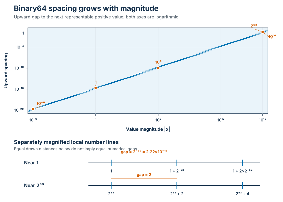
Both axes in Figure 1 are logarithmic because the displayed values and gaps span many orders of magnitude. The staircase is intentional: the absolute spacing is constant within each normal exponent interval and doubles at a power-of-two boundary. The two number lines are magnified independently; they compare local structure and do not share one linear scale.
The spacing is not a single fixed decimal resolution. Within each normal binary scale interval, the absolute spacing is fixed; when the exponent increases, the spacing grows. The relative spacing remains of a similar order throughout the normal range.
An ulp, or unit in the last place, describes spacing at a particular floating-point value. Python’s math.ulp(x) exposes this local scale. At \(x=1\), it returns approximately \(2.22\times10^{-16}\), which is also sys.float_info.epsilon: the gap between 1 and the next larger binary64 value.
Machine epsilon characterizes a format near 1. It is not a universal tolerance for comparing arbitrary results. The same absolute difference can be tiny at one scale, enormous at another, or decisive near a scientific threshold. Module 3 develops comparison rules that account for that context.
Rounding happens locally
For a basic arithmetic operation, a useful working model is:
- consider the exact mathematical result of the operation;
- if that result is representable, store it exactly;
- otherwise, select a nearby representable value according to the active rounding rule.
The usual IEEE 754 rule is round to nearest, ties to even. A result is rounded to the nearest representable value; an exact halfway case is resolved so that the least significant retained digit is even. Other rounding modes exist, but the course examples assume the usual default.
Rounding is local because it occurs after individual operations. A later operation receives the already-rounded operand; it does not have access to the discarded information. Consequently, rounding at an early stage may have no visible effect, may be offset by later rounding, or may influence the final result.
At \(x=2^{53}\), adjacent binary64 values are two units apart. The exact value \(x+1\) lies halfway between two representable values, so the default tie rule rounds it back to \(x\):
x + 1.0 == x      -> True
x + 2.0 == x      -> False
The value 1.0 has not become zero. It is too small to change the stored result at that scale. This is why a test such as x + small == x must be interpreted in terms of the format and the magnitude of x.
Numerical states at the limits
IEEE 754 formats reserve representations for values and states that do not fit the ordinary normal-number model.
| State | Meaning | Important behaviour |
|---|---|---|
| Normal finite number | A nonzero value represented with the format’s full significand precision | Most routine floating-point values are normal. |
| Subnormal number | A nonzero value smaller in magnitude than the smallest normal value | Subnormals provide gradual underflow, but retain fewer significant bits as they approach zero. |
| Positive or negative zero | A zero with a retained sign | 0.0 == -0.0 is true, but the sign can affect some functions and limiting operations. |
| Positive or negative infinity | A value beyond the finite range, or an explicitly constructed infinity | Arithmetic can propagate infinity; some operations involving infinities are invalid. |
NaN |
“Not a Number,” used for an invalid or indeterminate numerical result | NaN propagates through many operations and is not equal to itself. |
For binary64, the largest finite value is approximately \(1.80\times10^{308}\). A result whose magnitude is too large for the finite range overflows. Depending on the language, operation, and runtime policy, overflow may produce infinity, raise an exception, set a status flag, or issue a warning.
The smallest positive normal binary64 value is approximately \(2.23\times10^{-308}\). Smaller nonzero results may enter the subnormal range, where precision gradually decreases. A result too small even for that range rounds to a signed zero. These outcomes occupy the underflow region; underflow is not limited to the final transition to zero. IEEE 754 status signalling additionally depends on whether a tiny result is inexact.
Special values should be classified rather than hidden. In Python, math.isfinite, math.isinf, and math.isnan express the intended checks. Testing value == float("nan") does not work because every ordered comparison with NaN is false, equality with itself is false, and inequality is true. Language behaviour also matters: Python raises an exception for floating-point division by zero even though the underlying format includes infinities.
Real-number algebra is not always computational algebra
Associativity says that changing the grouping of additions does not change the result over the real numbers. Floating-point addition does not generally preserve that identity because each grouped operation can round differently. For example, let
a = 1e16
b = -1e16
c = 1.0
Then binary64 arithmetic in the course environment gives:
| Expression | Computed result |
|---|---|
(a + b) + c |
1.0 |
a + (b + c) |
0.0 |
In the first expression, a + b is exactly zero, so adding c produces one. In the second, adding c to b does not change the stored value at that scale; the subsequent addition therefore produces zero. Both expressions equal one in exact real arithmetic, but their sequences of intermediate floating-point operations differ.
This does not mean algebra is useless. It means an algebraic rewrite can change the computation, and the consequences must be checked rather than assumed.
Explaining the opening variance discrepancy
The centered variance formula first subtracts the mean. For the Module 1 data, the mean is \(100{,}000{,}010\ \mathrm{ns}\) and the centered values are \([-6,-3,3,6]\ \mathrm{ns}\). Its subsequent arithmetic therefore operates on quantities near the scale of the spread.
The shortcut formula computes a mean of squared timestamps and the square of the mean. Both intermediate values are near \(10^{16}\ \mathrm{ns}^2\), where adjacent binary64 values are \(2\ \mathrm{ns}^2\) apart. Each intermediate is rounded before they are subtracted. Although their exact difference is \(22.5\ \mathrm{ns}^2\), the rounded intermediates no longer retain enough information to recover that value, and their computed difference is \(22.0\ \mathrm{ns}^2\).
The two formulas are mathematically equivalent but not computationally equivalent in binary64 arithmetic. This explanation is consistent with the Module 1 evidence: changing the common timestamp offset increases the scale of the shortcut formula’s intermediates without changing the variance itself.
The example does not establish that every centered calculation is reliable for every input, nor that every algebraic rearrangement is harmful. It shows why an implementation must be evaluated as a sequence of finite-precision operations, not only as an expression over real numbers.
What this model does and does not establish
The spacing experiments, lost increment, changed evaluation order, and variance intermediates are all predicted by the finite-set model. That agreement gives us a coherent explanation rather than a collection of surprising outputs.
The model used here has deliberate limits:
- Except for the explicitly labelled format comparison, the numerical values shown assume IEEE 754 binary64 and the default rounding mode used by the published Python environment.
- Other types may have a different base, precision, range, or special-value policy.
- The notebook’s bfloat16 helper models a declared conversion path; it does not establish the arithmetic or performance of untested hardware or libraries.
- Languages, libraries, and compilers can differ in how they report exceptional states and in whether they combine particular operations.
- Knowing why two results differ does not determine whether the difference is acceptable for a scientific purpose.
The last point is essential. Floating-point arithmetic explains a source of discrepancy; it does not supply a validation threshold.
Questions to ask about a floating-point computation
- Which floating-point format or numeric type is being used?
- Does its allocation of significand and exponent bits provide enough local precision and range for the relevant values?
- Are the input values exactly representable, or are they rounded during conversion?
- What is the local spacing at the magnitudes of important inputs and intermediate results?
- Can a small contribution be rounded away when combined with a much larger value?
- Could an intermediate result overflow, become subnormal, or underflow to zero even if the final mathematical result is finite?
- Could regrouping or reformulating the operations change which information is retained?
- Are
NaN, infinity, and signed zero detected and handled according to the scientific meaning of the calculation?
Reflection questions
- Why can Python display
0.1even though the exact stored binary64 value is slightly different? - At \(x=2^{53}\), why does
x + 1.0 == xnot imply that1.0is zero? - Why can changing parentheses alter a floating-point sum?
- What is the difference between overflow and underflow?
- How does local spacing explain the failure of the shortcut variance formula?
- Why should
sys.float_info.epsilonnot be copied directly into every numerical comparison? - Why can bfloat16 represent \(10^{-20}\) as a normal value while binary16 rounds it to zero, even though both formats use 16 bits?
- Python normally prints the shortest decimal text that converts back to the same stored value. The display hides unnecessary digits; it does not claim that the decimal fraction is represented exactly.
- The spacing at that magnitude is two. The exact sum lies between representable values and rounds back to
xunder the default rule. - Each grouping creates a different sequence of intermediate results, and each intermediate may be rounded before the next operation.
- Overflow occurs when a magnitude is too large for the finite range. Underflow occurs when a nonzero magnitude is too small for normal representation and may produce a subnormal value or signed zero.
- The shortcut creates intermediate values near \(10^{16}\ \mathrm{ns}^2\), where the spacing is \(2\ \mathrm{ns}^2\). Rounding those values before their subtraction loses information needed to recover the exact variance.
- Machine epsilon describes spacing near one for a particular format. A defensible comparison must also account for the scale of the values and the accuracy required by the scientific question.
- Bfloat16 devotes eight bits to the exponent, giving it approximately the normal range of binary32. Binary16 uses only five exponent bits and spends more of its 16-bit budget on significand precision. Equal storage width does not imply equal range or spacing.
Takeaways
- Floating-point values form a finite, nonuniformly spaced approximation to the real numbers; precision and range are distinct.
- Binary16 and bfloat16 demonstrate that the same storage width can encode very different precision-and-range trade-offs; the format must be named.
- Conversion and arithmetic round locally, so small contributions can disappear and evaluation order can change a result.
- Subnormal numbers, signed zero, infinity, and
NaNare meaningful observable states that should be classified explicitly. - A finite-precision model can explain a discrepancy, but it cannot decide whether that discrepancy is scientifically acceptable.
Connection to the next module
We can now explain why two floating-point computations may differ. Module 3: Measuring And Comparing Numerical Error introduces absolute, relative, and mixed comparisons for deciding whether a difference matters at the relevant scale.