Module 4: Conditioning And Numerical Stability
Motivation
Suppose a computed result fails the comparison defined in Module 3. Increasing the tolerance would merely weaken the requirement; it would not identify what went wrong. A useful remedy depends on the cause.
Two causes are easy to confuse. The mathematical problem may be intrinsically sensitive, so small changes in measured or represented inputs necessarily produce large output changes. Alternatively, the problem may permit an accurate answer while the selected algorithm loses much more information than necessary. A third possibility is simpler: the program does not implement the intended algorithm.
These cases call for different responses. Better arithmetic cannot recover information absent from uncertain inputs, while better measurements do not fix an unreliable algorithm or an indexing defect.
Learning outcomes
After this module, you should be able to:
- describe conditioning as input-to-output sensitivity for a stated problem, input, norm, and scale;
- distinguish problem conditioning from algorithmic stability and implementation correctness;
- use controlled perturbations to estimate directional sensitivity;
- propagate small deterministic input bounds or standard uncertainties through a smooth model, while accounting for covariance and stating the assumptions behind the result;
- interpret forward error, backward error, and residuals as different questions;
- explain why a small residual need not imply a small forward error;
- select evidence and remedies that match the diagnosed source of error.
Connection to Module 3
Module 3 established how to measure a discrepancy and judge it against a defensible requirement. This module assumes those choices are already explicit: the reference, units, norm or scalar metric, and tolerance are known.
We now ask why the discrepancy occurs. Scale-aware error measures must come first because conditioning and stability compare relative sizes: input changes, output changes, forward errors, backward errors, and residuals. A diagnosis is meaningless if those quantities have not been defined.
Three questions, three objects
| Question | Object being assessed | Evidence |
|---|---|---|
| How sensitive is the answer to the input? | The mathematical problem at a specified input | Deliberate input perturbations, analytic bounds, or a condition estimate |
| Does the algorithm introduce more error than the problem requires? | The algorithm for a specified input range and arithmetic | Forward and backward error, precision changes, or comparison with a better formulation |
| Does the program perform the intended algorithm? | The implementation | Specification-based tests, known cases, invariants, and code review |
Conditioning belongs to the mathematical problem, not to a particular program. Stability describes an algorithm’s numerical behaviour; it is not the same as whether the source code is free of defects. A program can faithfully implement an unstable algorithm, or incorrectly implement a stable one.
Conditioning measures problem sensitivity
Consider a problem that maps input data \(b\) to a result \(x\). Change the input by \(\Delta b\) and observe a corresponding output change \(\Delta x\). A directional relative amplification is
\[ \kappa_\mathrm{obs} = \frac{\|\Delta x\|/\|x\|} {\|\Delta b\|/\|b\|}. \]
A norm is a rule that turns a vector into one nonnegative measure of its size. The norm and scaling are part of the definition. This module uses the maximum norm, \(\|v\|_\infty=\max_i|v_i|\): take the absolute value of every component and select the largest. For example, \(\|(-3,4,1)\|_\infty=4\). The vectors, norms, and scaling reference compares this choice with other common norms.
Here the maximum norm is applied to dimensionless, nondimensionalized quantities. If components have different units or meaningful scales, they must be scaled before one relative measure can be interpreted.
A formal local condition number describes the largest amplification over all sufficiently small perturbation directions. One experiment gives an observed directional amplification, not a proof of that worst case. It can nevertheless reveal severe sensitivity.
A well-conditioned problem has modest amplification for the perturbations that matter. An ill-conditioned problem can amplify input uncertainty or rounding so strongly that the requested output accuracy is unattainable. Conditioning is not a binary label: it depends on the input, the chosen output, the perturbation model, and the norm.
A two-equation sensitivity experiment
This experiment instantiates the preceding definition. For each fixed positive \(\delta\), define a mathematical map \(f_\delta:b\mapsto x\) by solving the dimensionless system
\[ \begin{aligned} x_1+x_2 &= b_1,\\ x_1+(1+\delta)x_2 &= b_2. \end{aligned} \]
The input is the right-hand-side vector \(b=(b_1,b_2)\); the output is the exact solution vector \(x=(x_1,x_2)\). The parameter \(\delta\) selects which map is being examined and is held fixed during each perturbation experiment. If \(\delta\) were itself uncertain, the coefficient data would also have to be included in the input, but that is a different conditioning question.
Use the baseline input
\[ b_\delta=(2,2+\delta), \]
for which \(f_\delta(b_\delta)=(1,1)\). Now change only the second component of the input by \(\eta\):
\[ \Delta b=(0,\eta), \qquad \widetilde b_\delta=b_\delta+\Delta b=(2,2+\delta+\eta). \]
Solving the perturbed system exactly gives
\[ \widetilde x_2=1+\frac{\eta}{\delta}, \qquad \widetilde x_1=1-\frac{\eta}{\delta}, \]
so \(\Delta x=(-\eta/\delta,\eta/\delta)\). In the maximum norm used above,
\[ \frac{\|\Delta b\|_\infty}{\|b_\delta\|_\infty} =\frac{|\eta|}{2+\delta}, \qquad \frac{\|\Delta x\|_\infty}{\|x\|_\infty} =\frac{|\eta|}{\delta}. \]
Substitution into the preceding definition connects the experiment directly to the observed directional amplification:
\[ \kappa_\mathrm{obs}=\frac{2+\delta}{\delta}. \]
The same absolute right-hand-side perturbation is used for each map, but its effect on the solution grows as \(\delta\) decreases. With \(\eta=10^{-16}\), high-precision decimal arithmetic gives:
| \(\delta\) | Relative RHS-input change | Relative solution-output change | Observed amplification |
|---|---|---|---|
| \(1\) | approximately \(3.33\times10^{-17}\) | \(10^{-16}\) | approximately \(3\) |
| \(10^{-12}\) | approximately \(5.00\times10^{-17}\) | \(10^{-4}\) | approximately \(2.00\times10^{12}\) |
Reducing \(\delta\) makes the two left-hand sides nearly identical, so the problem has little information with which to distinguish \(x_1\) from \(x_2\). For each table row, however, \(\delta\) is fixed and only the declared input \(b\) changes. The large output change is therefore evidence of sensitivity of the mathematical map, not binary64 rounding: the experiment uses high-precision decimal arithmetic and the amplification follows directly from the equations. It measures one perturbation direction, not the worst-case condition number.
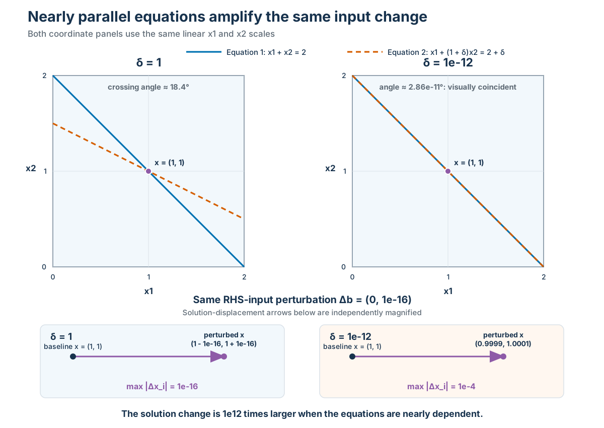
The upper panels use identical coordinate scales. The near overlap for \(\delta=10^{-12}\) is therefore the geometric evidence: the two equations constrain almost the same direction. Their small angular difference cannot be resolved at this scale. The lower displacement arrows are deliberately and independently magnified; their labels, rather than their drawn lengths, give the quantitative comparison. The same input perturbation produces a solution change \(10^{12}\) times larger in the nearly dependent system.
Propagation combines sensitivity with input information
Conditioning asks how strongly a mathematical model could amplify input changes. Propagation combines that sensitivity with a declared description of which input changes are possible or plausible.
The word error needs care here. For a synthetic test with a known exact input, the input error can be calculated. For measured data, the unknown true value is usually unavailable. What can be propagated is instead a stated input bound, standard uncertainty, covariance, probability distribution, or set of admissible values. These descriptions are not interchangeable.
Let a scalar result be
\[ y=f(x_1,x_2,\ldots,x_n). \]
For sufficiently small input changes and a differentiable model, first-order linearization gives
\[ \Delta y \approx \sum_{i=1}^n c_i\Delta x_i, \qquad c_i=\left.\frac{\partial f}{\partial x_i}\right|_{x_1,\ldots,x_n}. \]
The derivatives \(c_i\) are sensitivity coefficients. Their units convert a change in each input into a change in the output. They may be derived analytically, computed with automatic differentiation, or estimated with carefully scaled and checked numerical perturbations.
For small deterministic bounds \(|\Delta x_i|\le b_i\), adding the magnitudes of the linearized contributions gives the first-order estimate
\[ |\Delta y| \lesssim \sum_{i=1}^n |c_i|b_i. \]
This expression explains the familiar arithmetic rules:
| Operation | Small-change first-order estimate |
|---|---|
| \(y=a\mathbin{+}b\) or \(y=a-b\) | \(|\Delta y|\lesssim |\Delta a|+|\Delta b|\) |
| \(y=ab\) or \(y=a/b\) | \(|\Delta y/y|\lesssim |\Delta a/a|+|\Delta b/b|\) |
| \(y=a^p\) | \(|\Delta y/y|\lesssim |p|\,|\Delta a/a|\) |
The product, quotient, and power expressions are local approximations, not rigorous bounds for arbitrary input ranges. A rigorous deterministic envelope requires bounding the nonlinear remainder or evaluating the complete admissible input set with a justified method.
Worked example: density from bounded inputs
Suppose mass and volume are known only to lie in the ranges
\[ m\in[99.8,100.2]\ \mathrm{g}, \qquad V\in[39.7,40.3]\ \mathrm{cm^3}, \]
and the model is \(\rho=m/V\). At the nominal inputs, \(\rho=2.5\ \mathrm{g\,cm^{-3}}\). Because density increases with \(m\) and decreases with positive \(V\), the exact extrema over this rectangular input set occur at opposite corners:
\[ \frac{99.8}{40.3} \le \rho \le \frac{100.2}{39.7}, \]
or
\[ 2.47643 \le \rho \le 2.52393\ \mathrm{g\,cm^{-3}}. \]
The first-order relative estimate is
\[ \frac{|\Delta\rho|}{\rho} \lesssim \frac{0.2}{100.0}+\frac{0.3}{40.0} =0.0095, \]
which gives \(|\Delta\rho|\lesssim0.02375\ \mathrm{g\,cm^{-3}}\). The exact deviations are asymmetric: approximately \(-0.02357\) and \(+0.02393\ \mathrm{g\,cm^{-3}}\). The first-order result is a useful scale estimate here, but its slight miss at the upper endpoint shows why it must not be presented as an exact bound.
Covariance describes coupled input variation
Now make a different statement: suppose \(0.2\ \mathrm{g}\) and \(0.3\ \mathrm{cm^3}\) are standard uncertainties, rather than interval half-widths. Under a declared probabilistic input model, the standard uncertainty \(u(x_i)\) is the standard deviation assigned to the uncertain input \(X_i\) represented by the estimate \(x_i\).
Covariance describes whether two uncertain inputs tend to deviate from their means together. If \(\mu_i=\operatorname{E}[X_i]\) and \(\mu_j=\operatorname{E}[X_j]\), then
\[ \operatorname{Cov}(X_i,X_j) = \operatorname{E}\left[(X_i-\mu_i)(X_j-\mu_j)\right], \]
where \(\operatorname{E}\) denotes an average under the declared probability model. Positive covariance means that above-average values of the two inputs tend to occur together; negative covariance means that an above-average value of one tends to accompany a below-average value of the other. Zero covariance means that they are uncorrelated, but does not in general prove that they are independent.
Covariance has the product of the two inputs’ units, so its magnitude is not a unit-free measure of association. The corresponding correlation is
\[ \operatorname{Corr}(X_i,X_j) = \frac{\operatorname{Cov}(X_i,X_j)}{u(x_i)u(x_j)}, \]
which is dimensionless and lies between \(-1\) and \(1\). Covariance is the quantity needed in uncertainty propagation; correlation is often easier to interpret and can be converted to covariance when the two standard uncertainties are known.
The input covariance matrix collects every pairwise covariance:
\[ (\Sigma_x)_{ij}=\operatorname{Cov}(X_i,X_j). \]
Its diagonal entries are the input variances, \(\operatorname{Cov}(X_i,X_i)=u^2(x_i)\), while its off-diagonal entries describe coupled variation. For two inputs,
\[ \Sigma_x= \begin{bmatrix} u^2(x_1) & \operatorname{Cov}(X_1,X_2)\\ \operatorname{Cov}(X_1,X_2) & u^2(x_2) \end{bmatrix}. \]
Let the row vector \(J=[c_1,\ldots,c_n]\) contain the sensitivity coefficients. First-order propagation gives
\[ u_c^2(y)\approx J\Sigma_xJ^\mathsf{T} = \sum_{i=1}^n\sum_{j=1}^n c_i c_j\operatorname{Cov}(X_i,X_j). \]
If the inputs are independent, the off-diagonal covariance terms vanish and this reduces to
\[ u_c(y)\approx \sqrt{\sum_{i=1}^n\left(c_i u(x_i)\right)^2}. \]
For the density example, treating the stated values as independent standard uncertainties gives
\[ u_c(\rho) \approx 2.5\sqrt{ \left(\frac{0.2}{100.0}\right)^2+ \left(\frac{0.3}{40.0}\right)^2} =0.0194\ \mathrm{g\,cm^{-3}}. \]
This is not the deterministic interval calculated above, nor is it automatically a confidence interval. It is an estimated standard uncertainty under a different input model. Without assuming independence, the density variance contains the cross-term
\[ u_c^2(\rho) \approx c_m^2u^2(m)+c_V^2u^2(V) +2c_mc_V\operatorname{Cov}(M,V). \]
Here \(c_m=1/V\) is positive and \(c_V=-m/V^2\) is negative. Positive covariance between mass and volume therefore makes the cross-term negative and reduces this first-order variance; negative covariance increases it. A shared calibration or environmental effect can make inputs vary together, so assuming independence without evidence can make the propagated uncertainty wrong in either direction.
Relate propagation to conditioning
For nonzero scalar inputs and output, define componentwise relative sensitivity coefficients
\[ \kappa_i= \left|\frac{x_i}{y}\frac{\partial f}{\partial x_i}\right|. \]
Then the deterministic first-order estimate can be written as
\[ \left|\frac{\Delta y}{y}\right| \lesssim \sum_{i=1}^n \kappa_i\left|\frac{\Delta x_i}{x_i}\right|. \]
This is the connection between conditioning and propagation. The \(\kappa_i\) describe local amplification by the model; the declared input bounds or uncertainties describe how strongly each direction is excited. A large condition number is a warning about possible amplification, but it is not by itself an output uncertainty.
Know when first-order propagation is inadequate
Linearization is most credible when the model is smooth, the input uncertainty is small enough that one local derivative is representative, and the output is not near a singularity, branch change, or discontinuity. It should be checked when those conditions are doubtful.
For example, let \(Y=X^2\) with nominal input \(x=0\) and nonzero standard uncertainty \(u(x)\). The derivative at the nominal input is zero, so first-order propagation reports zero output uncertainty. That conclusion is false: plausible nonzero values of \(X\) produce positive values of \(Y\). Higher-order analysis or direct propagation is required.
Practical alternatives include:
- evaluate all corners when monotonicity or linearity proves that extrema occur there;
- use interval or optimization methods when a defensible deterministic bound is required, while checking dependency and overestimation effects;
- sample a justified joint input distribution and run the model repeatedly to approximate the output distribution;
- compare direct propagation with the linearized result to assess whether nonlinearity matters.
Monte Carlo propagation is often workable for complicated models, but it does not repair an unjustified input distribution, omitted correlation, model discrepancy, or insufficient sampling of rare events. It estimates a distribution; it does not automatically provide a rigorous worst-case bound.
Before the companion experiment
The sensitivity, stability, and residuals notebook reproduces the two-equation perturbation in high precision. Its live Jupyter version provides logarithmic controls for \(\delta\) and \(\eta\), while the published static page retains the reviewed fixed-scale figure. The notebook also compares two quadratic-root algorithms and constructs a candidate solution with a tiny residual but a large forward error.
Before running it, predict:
- how the amplification changes as \(\delta\) decreases;
- whether two algebraically equivalent root formulas have the same error;
- whether a candidate with a relative residual near \(10^{-13}\) must be close to the exact solution;
- which observation diagnoses the problem, the algorithm, or the implementation.
Preview the authoritative Quarto source from the repository root with:
quarto preview notebooks/04-sensitivity-stability-residuals.qmdThe complete site build also generates a downloadable Jupyter notebook.
Forward and backward error can be defined formally
Let \(d\) denote the supplied problem data and let \(S(d)\) be the set of exact solutions for those data. For a computed result \(\hat{x}\), define the forward error by
\[ e_{\mathrm{fwd}}(\hat{x};d) = \inf_{x\in S(d)} \rho_X(\hat{x},x), \]
where \(\rho_X\) measures distance in the solution space. If the problem has a unique exact solution \(x\), a common relative normwise choice is
\[ e_{\mathrm{fwd,rel}}(\hat{x};d) = \frac{\|\hat{x}-x\|_X}{\|x\|_X}, \qquad x\ne 0. \]
For a problem with multiple solutions, \(S(d)\) must contain the solutions that are acceptable for the scientific question. If a particular solution branch is intended, measuring the distance to any other branch could understate the error. An absolute or component-scaled measure is needed when a relative norm is undefined or inappropriate, for example when \(x=0\) or components have different units. When \(x\) is approximated by a high-precision or independent reference, the result is a measured forward-error estimate rather than the unknown exact forward error, and the reference must be justified.
The backward error instead measures distance in the data space. Define it by
\[ \eta(\hat{x};d) = \inf_{\Delta d\ \text{admissible}} \left\{ \rho_D(d,d+\Delta d) \;:\; \hat{x}\in S(d+\Delta d) \right\}. \]
Here \(\Delta d\) ranges only over admissible perturbations: changes that preserve whatever structure belongs to the problem, such as matrix symmetry, positive parameters, or fixed coefficients. The function \(\rho_D\) measures the size of the data change. For nonzero data, a common normwise relative choice is
\[ \rho_D(d,d+\Delta d)=\frac{\|\Delta d\|_D}{\|d\|_D}, \]
but an absolute or component-scaled measure may be more meaningful when some data are zero, have different units, or vary over very different scales. If no admissible perturbation makes \(\hat{x}\) exact, the backward error is infinite. Thus a numerical value for backward error is meaningful only together with its data, perturbation model, norm, and scaling.
For example, consider \(Ax=b\) with \(A\) held fixed. If \(r=b-A\hat{x}\), then \(\hat{x}\) exactly solves the nearby problem
\[ A\hat{x}=b+\Delta b, \qquad \Delta b=-r. \]
Under a relative normwise perturbation of the right-hand side, the backward error is therefore
\[ \eta_b(\hat{x};A,b) = \frac{\|r\|}{\|b\|}, \qquad b\ne 0. \]
Allowing perturbations in \(A\) as well would define a different backward error; that choice must be stated rather than assumed.
The two definitions expose the central contrast:
- forward error asks how far \(\hat{x}\) is from an acceptable exact solution;
- backward error asks how far the supplied data must move to make \(\hat{x}\) exact.
Stability measures algorithmic behaviour
An algorithm is backward stable for a stated class of inputs when every computed answer has a small backward error under the selected perturbation model. In floating-point analysis this is often expressed as \(\eta(\hat{x};d)\le C u\), where \(u\) is the unit roundoff and \(C\) is a modest factor that may depend on the problem size or input class. This asks whether the algorithm behaves as if it introduced only a small disturbance to the supplied data; it does not assert that the computed answer is close to the desired answer.
Backward stability does not guarantee small forward error. If the problem is ill-conditioned, a tiny backward error can be amplified into a large output error. Under suitable assumptions, the relationship is summarized by the first-order guide
\[ \text{relative forward error} \lesssim \text{condition number}\times\text{relative backward error}. \]
This is a reasoning pattern, not a universal equality. The precise bound depends on the problem, norm, perturbation model, and whether the changes are small enough for a local approximation.
Stability is also scoped. An algorithm may behave well for one input range and poorly for another, or in one arithmetic format and not another. Evidence from a constructed case supports a bounded claim rather than a timeless label.
Holding the problem fixed exposes algorithmic error
Consider the dimensionless quadratic
\[ x^2-Bx+1=0, \qquad B=10^8. \]
The smaller root can be evaluated directly as
\[ x_\mathrm{direct}=\frac{B-\sqrt{B^2-4}}{2}. \]
The product of the two exact roots is one. We can therefore compute the large root with the addition in the numerator and obtain the small root from its reciprocal:
\[ x_\mathrm{reformulated} =\frac{1}{(B+\sqrt{B^2-4})/2} =\frac{2}{B+\sqrt{B^2-4}}. \]
An 80-digit decimal reference, checked against a 100-digit recomputation, is approximately \(1.0000000000000001\times10^{-8}\). Binary64 results are:
| Method | Computed small root | Relative forward error | Relative coefficient backward error |
|---|---|---|---|
| Direct formula | \(7.450580596923828\times10^{-9}\) | approximately \(2.55\times10^{-1}\) | approximately \(1.46\times10^{-1}\) |
| Reformulated formula | \(1.0\times10^{-8}\) | approximately \(7.91\times10^{-17}\) | approximately \(3.95\times10^{-17}\) |
For a computed root \(\hat{x}\), the polynomial residual is \(p(\hat{x})=\hat{x}^2-B\hat{x}+1\). The coefficient backward-error measure used in the table is
\[ \eta_p= \frac{|p(\hat{x})|} {|\hat{x}|^2+B|\hat{x}|+1}. \]
It measures the relative coefficient perturbation needed to make the candidate an exact root under this component-scaled model. The problem and binary64 format are identical for both methods, but their forward and backward errors differ by many orders of magnitude. The algorithmic formulation therefore matters.
This example contains a recognizable arithmetic failure pattern. Module 5 names that pattern, shows where else it appears, and develops a broader set of mitigations. Here the purpose is to distinguish problem sensitivity from algorithmic behaviour.
Forward error, backward error, and residual answer different questions
Suppose \(Ax=b\) and a program returns \(\hat{x}\).
- Forward error compares \(\hat{x}\) with the desired solution \(x\). A relative max-norm measure is \(\|\hat{x}-x\|_\infty/\|x\|_\infty\). It requires a justified reference for \(x\).
- The residual is \(r=b-A\hat{x}\). It tests how well the candidate satisfies the supplied equations and has the units of \(b\).
- Backward error asks how much the input must change to make \(\hat{x}\) exact. If \(A\) is fixed, then \(\hat{x}\) exactly solves \(A\hat{x}=b-r\). The relative right-hand-side perturbation is \(\|r\|_\infty/\|b\|_\infty\).
A residual becomes interpretable only after scaling. “The residual is small” must say small relative to what and in which norm. Even a properly scaled small residual does not by itself bound forward error when the problem is ill-conditioned.
A small residual can accompany a wrong answer
Return to the two-equation system with \(\delta=10^{-12}\). The exact solution is \(x=(1,1)\), but consider the candidate \(\hat{x}=(0,2)\). Its diagnostics are:
| Diagnostic | Value |
|---|---|
| Relative forward error | \(1\) |
| Residual \(b-A\hat{x}\) | \((0,-10^{-12})\) |
| Relative right-hand-side backward error | approximately \(5.00\times10^{-13}\) |
The candidate is completely wrong in one component, yet it exactly solves the nearby system whose second right-hand side is \(2+2\times10^{-12}\) rather than \(2+10^{-12}\). The tiny input change is amplified by the ill-conditioned problem. This is why residual-based stopping criteria, introduced in Module 6, must be interpreted using conditioning and a meaningful scale.
Keep implementation defects separate
Stability analysis assumes that the implementation performs the algorithm being assessed. A sign error, wrong index, incorrect unit conversion, or unintended precision conversion can imitate unstable behaviour without saying anything about the intended algorithm.
Useful implementation evidence includes:
- exact or hand-checkable cases that exercise each code path;
- invariants and structural properties;
- comparison with an independently written implementation;
- tests that verify intermediate quantities, not only program termination;
- code review against the mathematical specification.
If the implementation is wrong, fix and retest it before drawing conclusions about conditioning or stability.
Match the experiment to the diagnosis
| Observation or experiment | What it can reveal | What it does not prove alone |
|---|---|---|
| Perturb inputs in high precision | Sensitivity inherent in the mathematical problem | Which finite-precision algorithm is best |
| Hold the problem fixed and compare algorithms | Avoidable differences caused by formulation | That the better method works for every input |
| Recompute in higher precision | Whether arithmetic effects contribute to the discrepancy | That the problem is well-conditioned or the implementation correct |
| Compute forward and backward errors | Whether the answer is accurate and whether it solves a nearby problem | The cause without a condition estimate |
| Check a scaled residual | Whether equations are nearly satisfied | Proximity to the desired solution on an ill-conditioned problem |
| Test known cases and invariants | Implementation fidelity and expected behaviour | A general stability theorem |
Use complementary experiments. A precision sweep, for example, can show that rounding contributes to an error, while a high-precision input perturbation can show that uncertain data would still be amplified even if arithmetic were exact.
Choose a remedy that matches the cause
For an ill-conditioned problem, possible responses include:
- improve the quality or quantity of input data;
- reformulate the mathematical question;
- nondimensionalize variables to remove artificial scale disparities, without claiming that scaling restores information absent from the inputs;
- change the requested output to one the data can support;
- introduce justified regularization, while documenting that it changes the problem;
- revise the claimed accuracy to reflect unavoidable input amplification.
Higher arithmetic precision can reduce rounding perturbations, but it cannot remove measurement uncertainty or create information absent from the data.
For an unstable or unsuitable algorithm, use a better formulation, a trusted numerical library, appropriate scaling, or—when justified—higher precision. Validate the replacement over the relevant input range rather than only on the case that originally failed.
For an implementation defect, correct the program and add a regression test that would have exposed the defect. Do not disguise it with a looser tolerance.
What the experiments establish and leave open
The two-equation experiment demonstrates directional sensitivity in a controlled, high-precision setting. It does not compute the full condition number for every perturbation direction. The density example demonstrates deterministic and covariance-based propagation for declared input descriptions; it does not establish that either description matches a real instrument. The quadratic experiment compares two algorithms on one exact coefficient set; it does not constitute a general proof of stability. The residual example demonstrates a logical possibility, not the output of a production solver.
Together, the examples establish the diagnostic distinctions:
- large output change under tiny high-precision input perturbation is evidence of problem sensitivity;
- large backward error for one algorithm but not an equivalent alternative is evidence of avoidable algorithmic error;
- a small residual or backward error can coexist with large forward error when the problem is ill-conditioned.
These conclusions remain separate from modelling error, discretization error, and the validity of a measurement-uncertainty model, which must be assessed with domain-specific evidence.
Questions to ask during diagnosis
- Which mathematical input-output map is being conditioned?
- Which input perturbations and output changes are scientifically meaningful?
- Are the inputs described by deterministic bounds, standard uncertainties, a joint distribution, or something else?
- Which inputs share calibration, sampling, or modelling effects and are therefore correlated?
- Which norm and scaling make the relative changes interpretable?
- Is first-order linearization adequate over the declared input range?
- Does sensitivity persist when the perturbation experiment uses higher precision?
- Does an equivalent algorithm reduce both forward and backward error?
- Is the residual scaled, and what relationship connects it to forward error?
- Has implementation fidelity been established independently?
- Does the proposed remedy target the problem, algorithm, or implementation?
Reflection questions
- Why is conditioning a property of a mathematical problem rather than a program?
- What does one observed amplification estimate establish about a condition number?
- How can a backward-stable result still have large forward error?
- Why does the high-precision two-equation experiment rule out binary64 rounding as the source of its large output change?
- What evidence attributes the quadratic-root discrepancy to the algorithmic formulation?
- Why is the residual of \((0,2)\) insufficient evidence that it approximates \((1,1)\)?
- Which remedies can address ill-conditioning, and which cannot recover uncertain input information?
- Why do a deterministic input interval and a standard uncertainty with the same numerical magnitude lead to different output statements?
- Why can omitting covariance invalidate propagated standard uncertainty?
- Give one reason why first-order propagation can fail.
- Conditioning describes how the exact answer changes when the mathematical input changes. It can be studied independently of any implementation.
- It measures sensitivity in one perturbation direction and can reveal severe conditioning, but it does not prove the worst-case amplification over all directions.
- A backward-stable result exactly solves a nearby problem. An ill-conditioned problem can map that tiny input change to a large output change.
- The calculations use high-precision decimal arithmetic, and the \(\eta/\delta\) amplification follows analytically from the exact equations.
- Both formulas solve the same polynomial in the same binary64 format. The reformulation has tiny forward and coefficient backward errors, while the direct formula has large errors under the stated measures.
- The nearly dependent equations cannot strongly distinguish the components. A relative right-hand-side perturbation near \(5\times10^{-13}\) makes \((0,2)\) exact even though its relative forward error is one.
- Better data, reformulation, a different supported output, justified regularization, or a revised accuracy claim can address the consequences. More arithmetic precision cannot reduce uncertainty already present in the inputs.
- A deterministic interval describes an admissible set and supports a range or bound. A standard uncertainty describes dispersion under a probabilistic model. Their propagation rules and interpretations are different.
- Covariance records input changes that occur together. The cross terms can either increase or decrease output variance, depending on the signs of the sensitivities and correlations.
- The model may be strongly nonlinear over the input range, cross a discontinuity or singularity, have a zero first derivative despite a nonzero higher-order effect, or receive input changes too large for a local approximation.
Takeaways
- Conditioning measures sensitivity inherent in a stated mathematical problem; stability measures the error behaviour of an algorithm; implementation correctness is a separate obligation.
- Forward error asks whether the answer is close, backward error asks whether it solves a nearby problem, and residual asks whether equations are nearly satisfied.
- A small backward error or residual does not guarantee a small forward error when the problem is ill-conditioned.
- Propagation combines model sensitivity with a declared input description; deterministic bounds, standard uncertainties, and probability distributions support different claims.
- First-order propagation is local. Check it against direct propagation when nonlinearity, correlation, singular behaviour, or decision thresholds may matter.
- Diagnose with controlled perturbations, algorithm comparisons, scaled diagnostics, and implementation tests, then choose a remedy that targets the identified cause.
Connection to the next module
Module 4 supplied the distinctions needed to diagnose numerical behaviour. Module 5: Common Numerical Failure Modes applies them to recurring patterns such as loss through subtraction, order-dependent accumulation, scaling problems, overflow, and underflow.